4.1. Continuum mechanics for fluids

Before entering the core of the matter, we should perhaps open with an informal discussion about what is a fluid, as opposed to a solid. When a strain is applied to a solid (for instance an elastic one), the latter develops a stress (like a spring) which resists to this strain. On the contrary, fluid are unable to withstand permanent deformations. They can only resist to relative deformations, by means of friction effects, in a way which dissipates energy (this is the concept of viscosity).

The fact that fluids are unable to resist shear stress explains that they naturally take the form of their containing vessel.

4.1.1. Kinematic description of fluids

In this first section, we present the main concepts from continuum mechanics involved in the kinematic study of a medium filled with a fluid, that is, in the analysis of the motion of the fluid without reference to the forces at its origin.

4.1.1.1. Eulerian description of fluids

Several descriptions are possible to account for the state of a fluid medium, but the perhaps most common one involves:

• The instantaneous velocity \(\textbf{u}(t,\textbf{x})\) of the fluid, depending on the time \(t\) and the considered point \(\textbf{x}\) in the medium;

• The pressure \(p(t,\textbf{x})\);

• The density \(\rho(t,\textbf{x})\) of the fluid at time \(t\) and point \(\textbf{x}\).

The velocity and pressure of the fluid are often referred to as the primitive variables. The Stokes system can actually be written in terms of different variables, leading to equivalent mathematical formulations, but lending themselves to different numerical methods.

4.1.1.2. Rate of strain and vorticity

The kinematic description of a fluid involves several quantities related to the velocity field \(\textbf{u}\). Let us assume (for simplicity only) that the velocity of the fluid has reached a steady state, so that it no longer depends on time. Then, a Taylor expansion about a given reference point \(\textbf{x}_0\) inside the medium yields, for points \(\textbf{x}\) close to \(\textbf{x}_0\):

\[\textbf{u}(\textbf{x}) = \textbf{u}(\textbf{x}_0) + \nabla \textbf{u}(\textbf{x}_0)(\textbf{x}-\textbf{x}_0) + {\mathcal O}(| \textbf{x} - \textbf{x}_0 |^2).\]

The Jacobian matrix \(\nabla \textbf{u}(\textbf{x}_0)\) in the previous identity can be broken down as the sum of its symmetric part \(D(\textbf{u}) := \frac{1}{2}(\nabla \textbf{u} + \nabla \textbf{u}^T)\) and its antisymmetric part \(\frac{1}{2}(\nabla \textbf{u} - \nabla \textbf{u}^T)\). This yields, if \(d=3\):

\[\textbf{u}(\textbf{x}) = \textbf{u}(\textbf{x}_0) + D(\textbf{u}) (\textbf{x}_0)(\textbf{x}-\textbf{x}_0) + \frac{1}{2}\mathbf{\omega}(\textbf{x}_0) \times (\textbf{x} - \textbf{x}_0) + {\mathcal O}(| \textbf{x} - \textbf{x}_0 |^2),\]

and if \(d=2\):

\[\textbf{u}(\textbf{x}) = \textbf{u}(\textbf{x}_0) + D(\textbf{u}) (\textbf{x}_0)(\textbf{x}-\textbf{x}_0) + \frac{1}{2}\omega(\textbf{x}_0) (\textbf{x} - \textbf{x}_0)^\perp + {\mathcal O}(| \textbf{x} - \textbf{x}_0 |^2),\]

where \(\textbf{h}^\perp = (-h_2,h_1)\) denotes the \(90^{\circ}\) counterclockwise rotate of a vector \(\textbf{h} = (h_1,h_2)\).

In the above equations, two important quantities appear:

• The rate of strain tensor \(D(\textbf{u}) = \frac{1}{2}(\nabla \textbf{u} + \nabla \textbf{u}^T)\) is the symmetric part of the Jacobian matrix of \(\textbf{u}\).

• The vorticity of the fluid is either a vector field, or a scalar field, depending on the space dimension:

  • If \(d=3\), the vorticity is the vector field \(\mathbf{\omega} : \Omega \to \R^3\) given by:

    \[\mathbf\omega = \nabla \times \textbf{u} = \left( \frac{\partial u_3}{\partial x_2} - \frac{\partial u_2}{\partial x_3}, \frac{\partial u_1}{\partial x_3} - \frac{\partial u_3}{\partial x_1}, \frac{\partial u_2}{\partial x_1} - \frac{\partial u_1}{\partial x_2} \right).\]

  • If \(d = 2\), it is the textit{scalar field} \(\omega : \Omega \to \R\) defined by:

    \[\omega = \frac{\partial u_2}{\partial x_1} - \frac{\partial u_1}{\partial x_2}.\]

The following two subsections allow to better appraise the physical meanings of these two fundamental concepts.

4.1.1.2.1. The rate of strain tensor

4.1.1.2.2. The vorticity of the fluid

The vorticity describes the tendency of the considered medium to rotate. Its definition is slightly different between the 2d and 3d cases.

To better understand the different effects of the two contributions in the above first-order term, let us assume that \(D(\textbf{u})(\textbf{x}_0) = 0\), and consider a particle starting from a point \(\textbf{x}_1\) close to \(\textbf{x}_0\). Then, the trajectory of the particle approximately satisfies the following ordinary differential equation:

\[\begin{split}\left\{ \begin{array}{cl} \mathring{\textbf{x}}(t) = \frac{1}{2}\mathbf\omega(\textbf{x}_0) \times (\textbf{x}(t)-\textbf{x}_0)& \text{for } t >0\\ \textbf{x}(0) = \textbf{x}_1. \end{array} \right.\end{split}\]

This is the motion of a rotation with axis \(\frac{1}{| \mathbf\omega(\textbf{x}_0) |}\mathbf\omega(\textbf{x}_0)\), and angular velocity \(\frac{1}{2}\mathbf\omega(\textbf{x}_0)\).

4.1.1.3. Streamlines and the stream function

Streamlines

It is the trajectory \(t \mapsto \textbf{x}(t)\) over a time period \((0,T)\) of a particle immersed in the fluid, occupying a given position \(\textbf{x}_0\) at time \(t= 0\), as it is driven by the velocity field \(\textbf{u}\). This trajectory is characterized by the ordinary differential equation:

\[\begin{split}\left\{ \begin{array}{cl} \mathring{\textbf{x}}(t) = \textbf{u}(t,\textbf{x}(t)) & \text{for } t \in (0,T), \\ \textbf{x}(0) = \textbf{x}_0. \end{array} \right.\end{split}\]

In particular, the trajectory lines are tangential to the velocity \(\textbf{u}(t,\textbf{x})\) of the fluid, see Fig. 4.1.

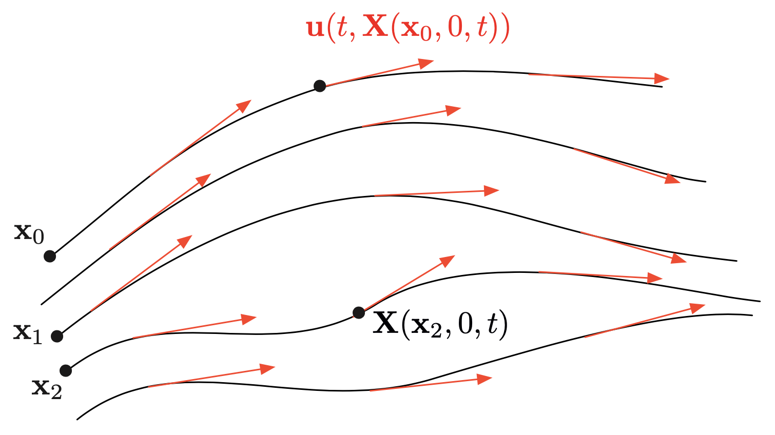
Fig. 4.1 Several streamlines, associated to different particles immersed in a fluid with velocity \(\textbf{u}(t,\textbf{x})\).

In the following, so as to emphasize the dependence on the initial position, we shall denote by \(t \mapsto \textbf{X}(\textbf{x}_0,0,t)\) the above trajectory.

The stream function

We now discuss a quite important concept which in particular allows for a very convenient way to vizualize flows in \(2d\). We restrict ourselves to the particular, two-dimensional situation where the flow is steady (that is, \(\textbf{u}\) does not depend on time), and the boundary conditions satisfied by the flow are such that:

\[\textbf{u} \cdot \n = 0 \text{ on } \partial \Omega.\]

We then define \(\psi\) to be such that:

\[\textbf{u} = \left( -\frac{\partial \psi}{\partial x_2} , \frac{\partial \psi}{\partial x_1} \right).\]

Assuming \(\Omega\) to be simply connected, such a function can be proved to exist, and to be unique up to constant. Now because of the boundary condition, we see that \(\psi\) is constant on \(\partial \Omega\). Taking the curl of the above equation, we have:

\[\Delta \psi = \nabla \times \textbf{u}.\]

We also observe that, denoting by \(\mathbf{\tau} := (-n_2,n_1)\) the tangent vector to \(\partial \Omega\) oriented counterclockwise (i.e. the 90 rotate of \(\mathbf{n}\)), it follows that:

\[\frac{\partial \psi}{\partial\mathbf{ \tau}}= -\textbf{u} \cdot \mathbf{n} \text{ on }\partial \Omega.\]

Therefore, in our case where \(\textbf{u} \cdot \mathbf{n}\), \(\psi\) is a constant on \(\partial \Omega\), which can be set to \(0\).

The above is a standard Laplace equation, which can be solved by standard means.

The main interest of the stream function lies in that the characteristic curves of the flow are included in the isolines of the stream function. Indeed, let \(t \mapsto \textbf{x}(t)\) be a characteristic curve of the flow, that is:

\[\begin{split}\left\{\begin{array}{cl} \mathring{\textbf{x}}(t) = \textbf{u}(\textbf{x}(t)) & \text{for } t \in (0,T), \\ \textbf{x}(0) = \textbf{x}_0& \end{array} \right.\end{split}\]

Then, the chain rule yields:

\[\frac{\d}{\d t}\left( \psi(\textbf{x}(t))\right) = \nabla \psi(\textbf{x}(t)) \cdot \textbf{u}(\textbf{x}(t)) = \left( - \frac{\partial \psi}{\partial x_1} \frac{\partial \psi}{\partial x_2} + \frac{\partial \psi}{\partial x_2} \frac{\partial \psi}{\partial x_1}\right)(\textbf{x}(t)) = 0.\]

Remark 4.1

• When it no longer holds that \(\textbf{u} \cdot \n = 0 \) on \(\partial \Omega\), it is still possible (and actually not much more complicated) to calculate the stream function. Indeed, the boundary condition \(\psi = 0\) on \(\partial \Omega\) is replaced by:

  \[\psi(s) = F(s),\]

  where \(s\) denotes arclength on \(\partial \Omega\) and \(f\) is one antiderivative for \(-\textbf{u} \cdot \n\).

• The theory could be partially extended to the 3d case, as far as the stream function is considered, but not as satisfactorily. We refer to Chap. 1 in [CM90] for a discussion of this subject.

4.1.2. Stresses

4.1.2.1. The Cauchy stress tensor

The Cauchy stress tensor \(\sigma(t,\x)\) has the following physical interpretation. Let \(\n\) be a direction of space; then the (vector) force \(\T^{(\n)}\) applied on the face oriented by \(\n\) of a very small cube-shaped piece of the medium around \(\x\) is: $$ \T^{(\n)} = \sigma(t,\x) \n.$$ Using Cartesian coordinates, this means that \(\sigma_{ij}(t,x)\) is the \(i^{\text{\rm th}}\) component of the force applied on the face with normal vector \(\e_j\) of a small cube around \(\x\); see \cref{fig.stresstensor} for an illustration.

begin{figure}[h] centering includegraphics [width=0.4textwidth]{figures/stresstensor} caption{it The Cauchy stress tensor as a descriptor of the efforts at play inside the medium.} label{fig.stresstensor} end{figure}

It is a non trivial consequence of the law of balance of momentum that the Cauchy stress tensor is symmetric, and we admit the result:

\begin{theorem} The Cauchy stress tensor is symmetric: \(\sigma_{ij} = \sigma_{ji}\), \(i,j=1,...,d\). \end{theorem}

The stress tensor may be decomposed as: $$ \sigma = s - p \I,$$ where: \begin{itemize} \item The scalar field \(p = - \frac{1}{3}\div \sigma\) is the pressure; roughly speaking, the contribution \(-p \I\) to the Cauchy stress tensor is responsible for the local change of volume; it is often referred to as the \textit{hydrostatic stress tensor}. \item The tensor field \(s\) is the \textit{deviatoric stress tensor}; this part is responsible for the distortion of a portion of medium, at constant volume. \end{itemize}

4.1.2.2. The law of balance of momentum

begin{proposition} The law of balance of momentum reads: $$ -div sigma = bm{f}.$$ end{proposition}

Considering inertia effects, we arrive at the law of balance of momentum in the context of incompressible fluids: $$ \frac{\partial \u}{\partial t} + (\u \cdot \nabla ) \u - 2\nu \div(D(\u)) + \nabla p = \bm{f}.$$ The term \((\u \cdot \nabla ) \u = (\nabla \u) \u\) is the vector whose entries are:

\[((\u \cdot \nabla) \u)_i = \sum\limits_{j=1}^d{u_j \frac{\partial u_i}{\partial x_j}} , \:\: i =1,...,d.\]

4.1.2.3. Boundary conditions

Often, the domain \(\Omega\) where the study is carried out is limited in space, and it is mandatory to supply the information about what happens at the boundary with the outer medium. Mathematically, this takes the form of conditions imposed at the boundary \(\partial \Omega\). These may be of different natures depending on the context.

No slip boundary conditions

No slip boundary conditions \(\u = \bz\) on \(\partial \Omega\).

The condition that \(\u \cdot \n\) is quite natural: this amounts to requiring that the boundary where the condition applies is impermeable, and cannot be crossed by the fluid.

The condition \(\u \cdot \mathbf{\tau}\) may seem odd at first glance. Why would the fluid stick to the boundary of the cavity?

Slip boundary conditions, with or without friction

Slip without friction boundary conditions \(\u \cdot \n = 0\) and \(\sigma \cdot \n =\bz\) (or not).

Pressure like boundary conditions

As we shall see, it is not mathematically correct to impose directly boundary conditions on the pressure, of the form \(p = p_0\) on some portion of \(\partial \Omega\). Instead, pressure boundary conditions are of Neumann type: \(\sigma \n = -p_0 \n\).

Surface tension at the interface between two different fluids

We now consider the following situation: a domain \(D\) is filled with two immiscible fluids, with different viscosities \(\nu_0, \nu_1\), occuping the respective subdomains \(\Omega_0 \subset D\) and \(\Omega_1 := D \setminus \overline{\Omega_0}\). We denote by \(\n\) the unit normal vector to the interface \(\Gamma := \partial \Omega_0\), pointing outward \(\Omega_0\), and we denote by \(\kappa\) the mean curvature of \(\Gamma\); see \cref{fig.bifluid} for an illustration.

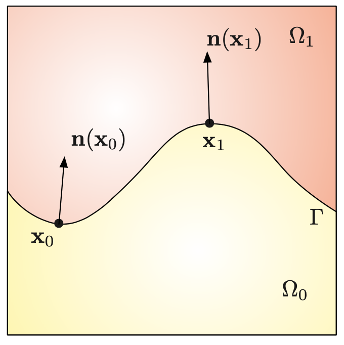
Fig. 4.2 Model situation of a bifluid situation. Here, the mean curvature \(\kappa\) is negative at \(\x_0\) and positive at \(\x_1\).

On account of the cohesive forces of particules of the same fluid, it is more beneficial for the fluid to minimize the contact surface between both fluids. In other terms, a portion \(G \subset \Gamma\) of the interface undergoes an additional force which drives it towards minimizing its area: $$ \bm{f} = -\int_{G}{\gamma \kappa \n \:ds}.

\[ The effect in terms of boundary conditions is that: \]

[\u](\x) = 0 \text{ and } [\sigma] \n(\x) = \gamma \kappa(\x) \n(\x), $$ where we denote by \([\alpha] := \alpha_1 - \alpha_0\) the jump of a quantity which is discontinuous across \(\Gamma\), taking values \(\alpha_0\), \(\alpha_1\) in \(\Omega_0\), \(\Omega_1\), respectively. The parameter \(\gamma>0\) featured in the above interface condition is a constant which depends on the physical properties of the two fluids (and in particular, of the intensity of the aforementioned cohesive forces).

We refer to Section 2.2 about the notion of mean curvature.

4.1.3. Rheology and constitutive laws

4.1.4. Boundary conditions