2.2. Calculating curvature

This section is devoted to the quite subtle notion of curvature of a curve, appraising how fast a point travelling on the latter changes direction, and its practical calculation. We first recall a few basic facts about curvature in Section 2.2.1, before describing its practical calculation with \(\texttt{FreeFem}\) in Section 2.2.2. The notion of curvature being significantly more involved in higher space dimensions, we focus on the 2d case.

2.2.1. Definition of curvature

Throughout this section, we consider a 2d curve \(\gamma\); with a small abuse of language, this terminology designates at the same time:

• A mapping \(\gamma: [a,b] \to \R^2\) between a parameter \(t\) in some interval \([a,b]\) and a point \(\gamma(t)\) in the 2d plane;

• The geometric locus of points formed by this mapping, i.e. the image \(\gamma([0,T])\).

The curve \(\gamma\) may be open (i.e. \(\gamma(a) \neq \gamma(b)\)) or closed (i.e. \(\gamma(a) = \gamma(b)\)).

Note that multiple parametrizations describe the same geometric object: for instance, if \(\alpha: [\widetilde{a},\widetilde{b}] \to [a,b]\) is a smooth bijective mapping, \(\widetilde{\gamma} = \gamma \circ \alpha: [\widetilde{a},\widetilde{b}] \to \R^2\) is another parametrization for \(\gamma\).

Let us first define first-order quantities related to \(\gamma\).

Definition 2.1

Let \(\gamma: [0,T] \to \R^2\) be a curve of class \(\calC^1\).

• The velocity of \(\gamma\) is the derivative \(\gamma^\prime : [0,T] \to \R^2\).

• The curve \(\gamma\) is called simple when \(\gamma^\prime\) does not vanish on \([0,T]\).

• The unit tangent vector \(\tau(\x)\) to \(\gamma\) at a point \(\x = \gamma(t)\) where \(\gamma^\prime(t) \neq 0\) is:

  \[\forall \x = \gamma(t), \: t\in (0,T), \quad \tau(\x) = \frac{\gamma^\prime(t)}{\lvert\gamma^\prime(t) \lvert}.\]

• The arc length of \(\gamma\) is the function \(s: [0,T] \to \R\) measuring the length from the initial value \(t=0\):

  \[\forall t \in [0,T], \quad s(t) = \int_0^t \lvert \gamma^\prime(u)\lvert \:\d u.\]

  One can prove that a simple curve \(\gamma\) may always be parametrized by its arc length, so that \(\gamma\) has constant, unit velocity:

  \[\forall \x = \gamma(t), \: t\in (0,T), \quad \lvert \gamma^\prime(t) \lvert =1. \]

The velocity \(\gamma^\prime(t)\) and the arc length \(s(t)\) of \(\gamma\) both depend on the chosen parametrization. On the contrary, the tangent vector \(\tau(\x)\), giving the orientation of the tangent line to \(\gamma\) passing through a point \(\x\) on \(\gamma\), only depends on the parametrization up to a sign, indicating the orientation of the curve, i.e. the sense of travel. These notions are illustrated on Fig. 2.2.

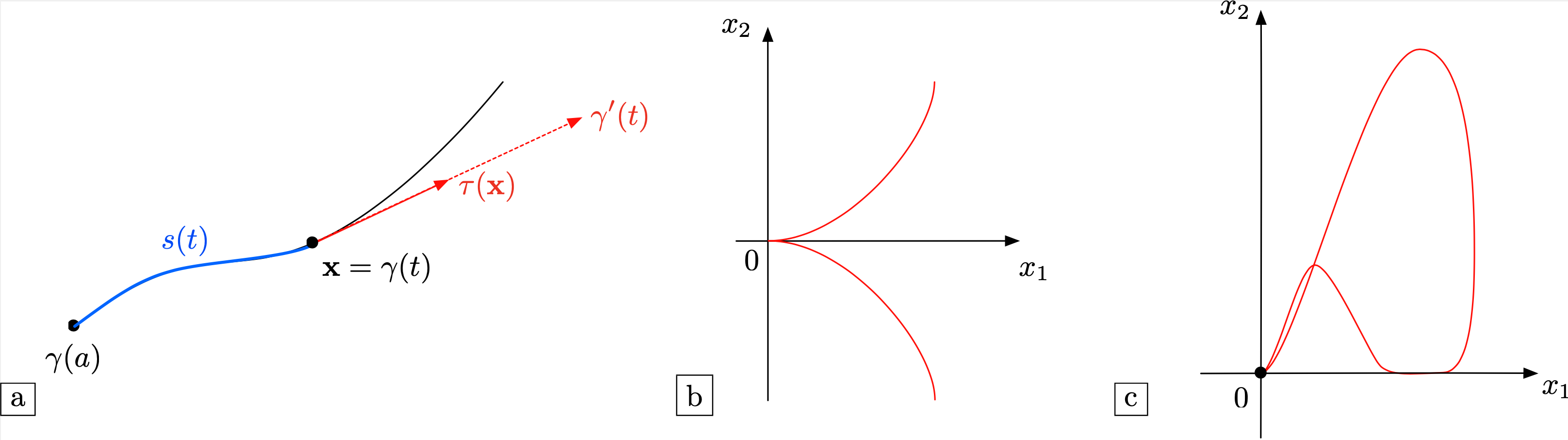
Fig. 2.2 \((\)a) Illustration of the first-order quantities attached to a curve \(\gamma\); (b,c) Two different pathologies featured by non simple curves : (b) The curve \(\gamma(t) = (t^2,t^3)\); (c) The curve \(\gamma(t) = \left(\frac{\cos^2 t}{2+\sin(2t)},\frac{\sin^4 t}{2+\sin(2t)}\right)\).

Let us now turn to the second-order features of a curve \(\gamma: [a,b]\to \R^2\) of class \(\calC^2\). The acceleration vector of \(\gamma\) is the second-order derivative \(\gamma^{\prime\prime} : [a,b] \to \R^2\) of the parametrization.

Definition 2.2

Let \(\gamma: [0,T] \to \R^2\) be a simple curve of class \(\calC^2\), parametrized by arc length. The curvature \(\kappa(\x)\) at the point \(\x = \gamma(t)\) is defined by

\[k(\x) = \lvert \gamma^{\prime\prime}(t) \lvert. \]

To get an insight about curvature, let us assume that \(\gamma\) is parametrized by arc length and let \(\x_0 = \gamma(t_0)\) be a point on \(\gamma\). A Taylor expansion of \(\gamma\) around \(t_0\) yields:

\[\gamma(t) \approx \gamma(t_0) + (t-t_0)\gamma^\prime(t_0) + \frac12 (t-t_0)^2 \gamma^{\prime\prime}(t_0). \]

Here,

• The vector \(\gamma^\prime(t_0) = \tau(\x_0)\) is the unit tangent vector to \(\gamma\) at \(\x_0\);

• The acceleration \(\gamma^{\prime\prime}(t_0)\) is orthogonal to \(\tau(\x_0)\), since

  \[\lvert \gamma^\prime(t)\lvert^2 = 1 \quad\Rightarrow \quad \gamma^\prime(t) \cdot \gamma^{\prime\prime}(t) = 0.\]
  We denote by \(\n_\gamma(\x) = \frac{\gamma^{\prime\prime}(t_0)}{\lvert \gamma^{\prime\prime}(t_0) \lvert}\) the unit normal vector to \(\gamma\) at \(\x_0\).

With these notations, the above expansion rewrites:

\[\gamma(t) \approx \x_0 + (t-t_0)\tau(\x_0) + \frac12 (t-t_0)^2 k(x_0) \n_\gamma(\x_0). \]

This expansion reflects the local behavior of \(\gamma\) near \(\x_0 = \gamma(t_0)\): at first order, \(\gamma\) follows the tangent direction \(\tau(\x_0)\). Its normal deviation is encoded in the second-order term: the larger the curvature \(k(\x_0)\), the faster it is; see Fig. 2.3 for an illustration.

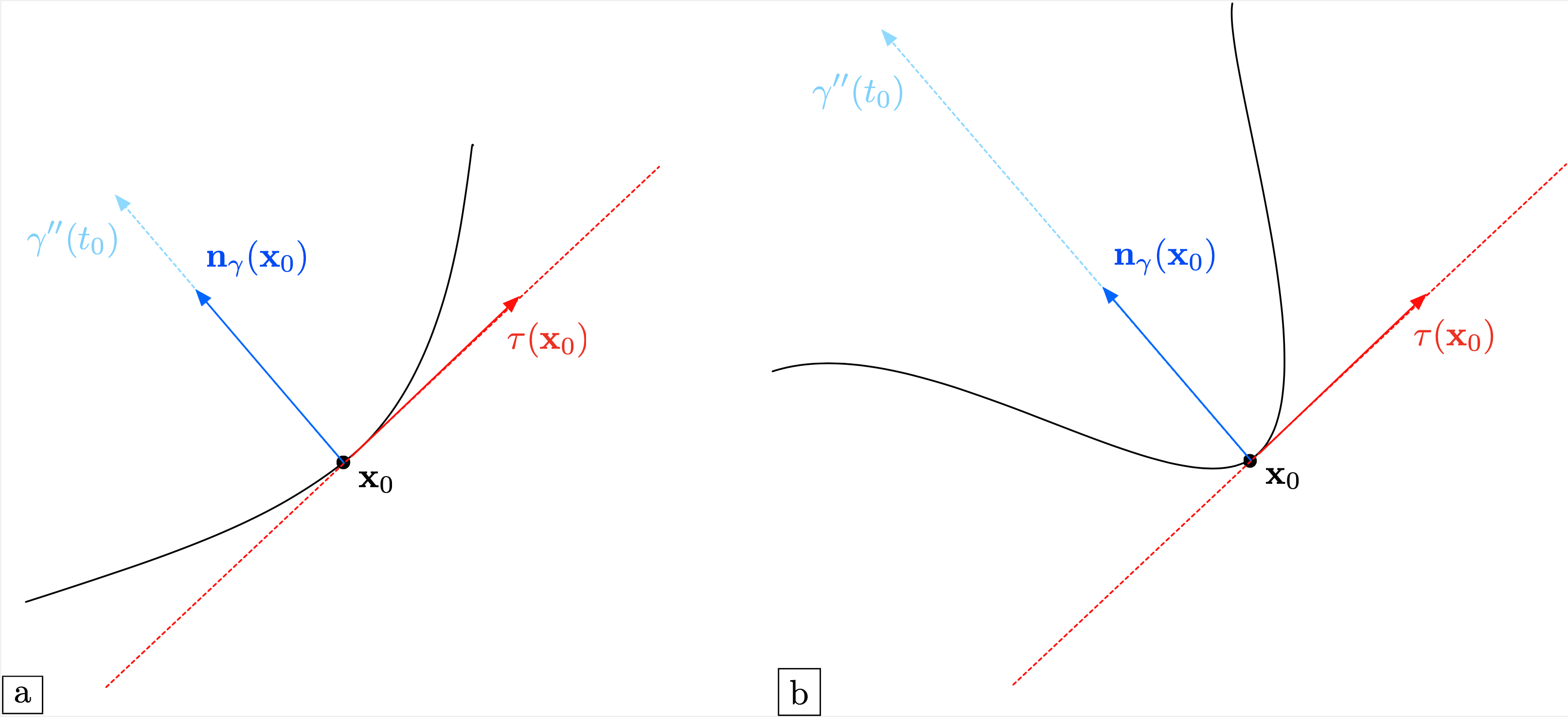
Fig. 2.3 Illustration of the second-order quantities attached to a curve \(\gamma\); (a) A situation where the curvature \(k(\x_0)\) is relatively small; (b) A situation where \(k(\x_0)\) is large.

The curvature \(k(\x)\) is an unsigned quantity. It is customary to endow it with a sign in the particular situation where \(\gamma\) is closed, and thus delimits an interior domain \(\Omega \subset \R^2\). In this situation, let \(\n\) be the unit normal vector to \(\gamma\) pointing outward \(\Omega\), whose orientation may differ from that of the normal vector \(\n_\gamma\) defined above. We define the oriented curvature \(\kappa(\x)\) of \(\gamma\) at \(\x\) by:

\[\kappa(\x) = -\gamma^{\prime\prime}(s) \cdot \n(\x);\]

in other terms, \(\kappa(\x) = \pm k(\x)\), where the sign is that of the product \(-\n(\x) \cdot \n_\gamma(\x)\). Note that the oriented curvature is positive when \(\gamma\) is locally convex near \(\x\), positive otherwise, see Fig. 2.4.

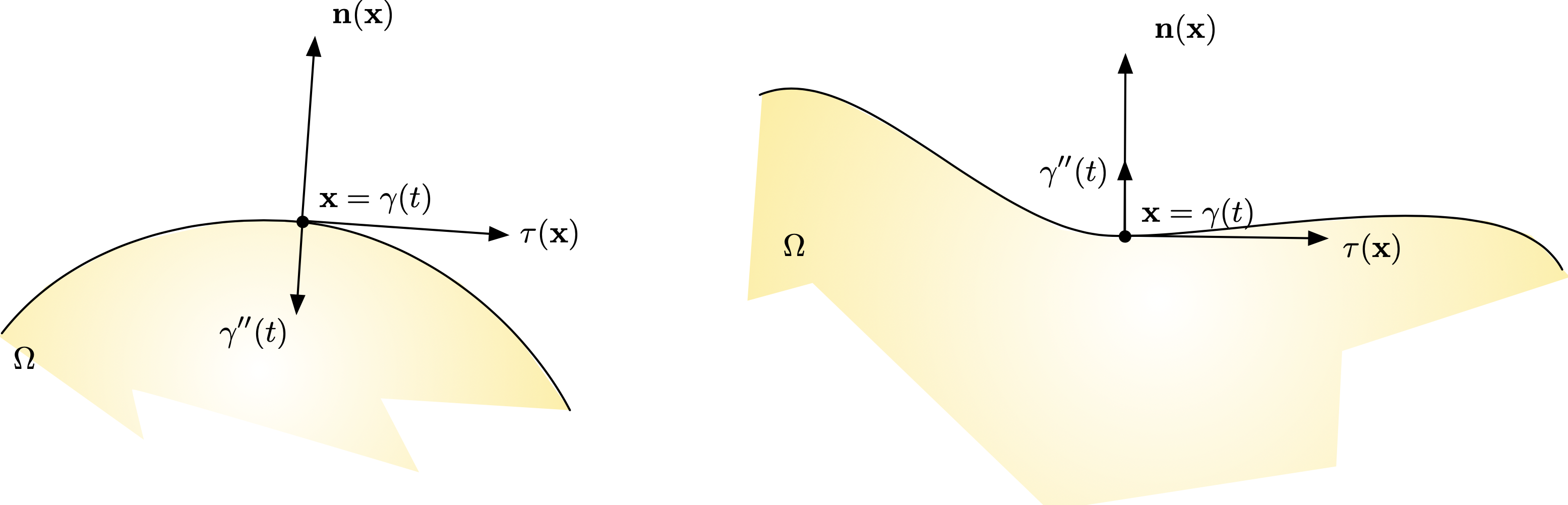
Fig. 2.4 (Left) The domain \(\Omega\) is convex near \(\x\): \(\kappa(\x) > 0\); (right) \(\Omega\) is concave near \(\x\): \(\kappa(\x) < 0\).

Example 2.1

Let \(\Omega = B(\bz,R)\) be the disk centred at the origin \(\bz\), with radius \(R\). The curvature \(\kappa(\x)\) at any point \(\x \in \partial \Omega\) equals \(\frac{1}{R}\), i.e. the larger the disk, the more "flat" its boundary appears.

2.2.2. Calculation of the mean curvature from a mesh

Let \(\Omega\) be a smooth bounded domain, equipped with a mesh \(\calT_h\). We aim to calculate the mean curvature \(\kappa\) at the points \(\x\) of the boundary \(\partial \Omega\).

The first step to achieve this goal is to approximate the unit normal vector \(\n\) to \(\partial\Omega\). Let \(\x_{i-1}\), \(\x_i\) and \(\x_{i+1}\) be three successive vertices on the discrete boundary \(\partial \Omega\), enumerated in counterclockwise order. The tangent vector \(\t(\x_i)\) to \(\partial \Omega\) at \(\x_i\) is approximated as:

\[\tau(\x_i) \approx \frac{\x_{i-1}-\x_{i+1} }{\lvert \x_{i-1}-\x_{i+1} \lvert}.\]

The normal vector \(\n(\x_i)\) is then obtained as the clockwise \(90\) rotate of \(\tau(\x_i)\); see Fig. 2.5.

In \(\texttt{FreeFem}\), the normal vector \(\n\) can be calculated in a simpler way, which uses the reserved keywords N.x and N.y. These can only be used inside a one-dimensional integral int1d(Th) call, and they represent the components of the normal vector field to the considered boundary. The following trick allows to calculate (an extension to \(\Omega\) of) them as \(\P_1\) Finite Element functions on \(\calT_h\):

/* Calculation of the normal vector to a meshed interface */
/* Finite element spaces and functions */
fespace Ph(Th,P1);
Ph nx,ny,norm;

/* Calculation of the normal vector to all borders of the mesh */
real EPS = 1.e-5;
varf normalx(u,v) = int1d(Th)(N.x*v);
varf normaly(u,v) = int1d(Th)(N.y*v);

nx[] = normalx(0,Ph);
ny[] = normaly(0,Ph);
norm = sqrt(nx^2+ny^2+EPS^2);
nx = nx/norm;
ny = ny/norm;

Once \(\n(\x_i)\) is available, the following approximation formula allows to calculate the mean curvature \(\kappa(\x_i)\):

\[\frac{1}{\kappa(\x_i)} \approx - \frac{1}{4} \left( \frac{ (\x_{i-1}- \x_{i}) \cdot (\x_{i-1}- \x_{i}) }{\n(\x_i) \cdot (\x_{i-1}- \x_{i}) } + \frac{ (\x_{i+1}- \x_{i}) \cdot (\x_{i+1}- \x_{i})}{\n(\x_i) \cdot (\x_{i+1}- \x_{i}) } \right).\]

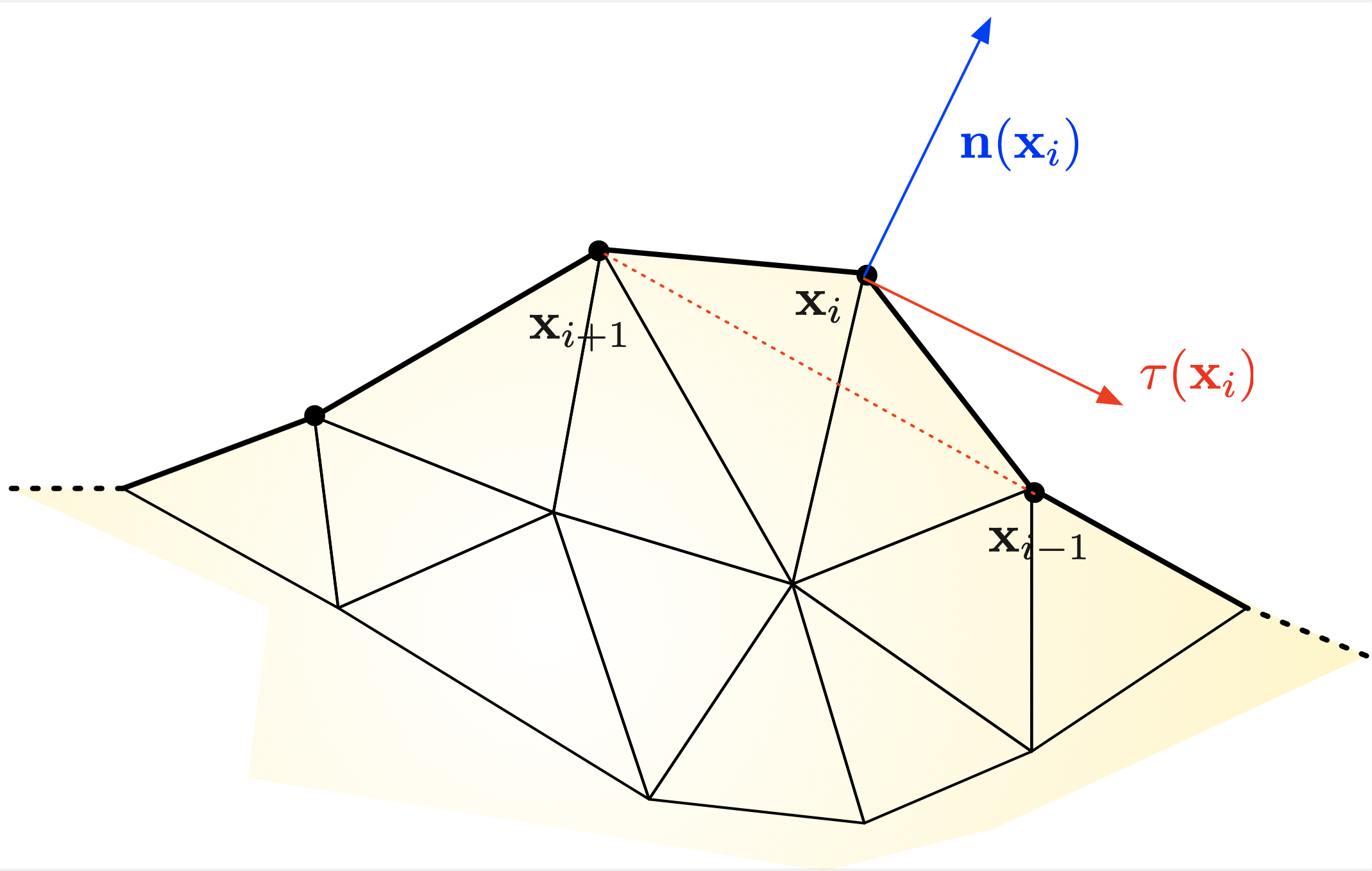
Fig. 2.5 Approximation of the curvature of a domain \(\Omega\) from a meshed discretization.

This idea is implemented in the function \(\texttt{curvatureFromMesh}\), contained in the independent module curvature.idp, which is called as follows:

/* Calculation of the mean curvature kappa from the datum of the normal vector (nx,ny) */
curvatureFromMesh(Th,nx[],ny[],kappa[]);

Exercise

Use these \(\texttt{FreeFem}\) recipes to:

1. Calculate the mean curvature of the unit ball; compare the result with the theoretical value \(\kappa=1\), see example 2.1.

2. Calculate the mean curvature of an ellipse with semi-axes \(0.1\) and \(0.2\).

A numerical result is presented in Fig. 2.6, and the associated code can be downloaded here.

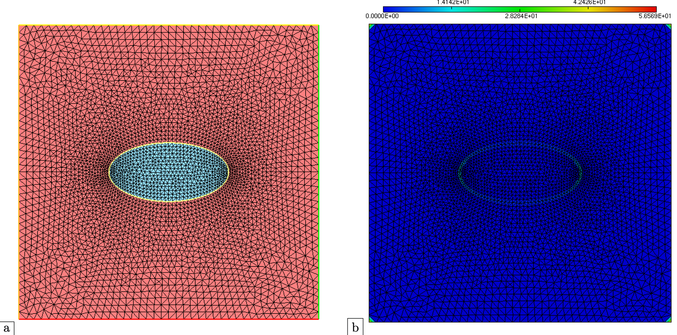
Fig. 2.6 \((\)a) Mesh of a box, containing a subdomain shaped as an ellipse; (b) Approximation of the curvature of all the boundaries of the mesh (including those of the bounding box).

Remark 2.1

The curvature of the boundary \(\partial\Omega\) of a domain \(\Omega\) can be calculated in a different fashion when the latter is represented by a level set function, as we shall see in the next Section 2.5.2.2.