3.1. An introduction to linear elasticity
This section deals with the physical model of linear elasticity describing the displacement of mechanical structures. Elasticity generally refers to the ability of an object to deform under the effect of loads, and to return to its exact initial configuration when they cease to be applied.
We consider particular instances of such situations, that hinge on two simplifying assumptions:
When the applied load is sufficiently small, so is the deformation, and the regime is linear.
We restrict ourselves to considering time-independent situations. After a transient regime, the situations is assumed to have reached a state of equilibrim.
The classical model of linear elasticity builds on three ingredients:
The first ingredient is kinematics, i.e. a description of the elastic body and its deformation, without making any reference to the efforts that have caused the latter. This is studied in Section 3.1.2.
The second ingredient is a model for efforts. They key concept in this respect is that of Cauchy’s stress tensor, which is discussed in Section 3.1.3.
The last ingredient is a connection between efforts and deformations: a constitutive law, depending on the mechanical characteristics of the elastic material, relates the applied stresses on a structure with the induced deformation. This is discussed in Section 3.1.4.
The reader primarily interested in the mathematical formulation of linear elasticity can directly jump to Section 3.1.6. Eventually, much intuition about mechanical structures can be gleaned by adopting an energy viewpoint. This is dicussed in Section 3.1.7.
When it comes to the description of a medium \(\Omega\), two paradigms are available:
The Lagrangian point of view assumes a reference configuration \(\widehat{\Omega}\) (for instance, the state of \(\Omega\) at rest, or at the initial time of study).
The Eulerian point of view considers all quantities of interest at the time \(t\) and point \(\x \in \Omega\) of interest.
While the former point of view is generally adopted in the field of structural mechanics, it is customary to rely on the latter in fluid mechanics.
3.1.1. Notations regarding vectors and tensors
Before getting into the core of the matter, let us set some notations. Let \(\sigma, \tau\) be two second-order tensors, i.e. mappings on \(\Omega\) whose values \(\sigma(\x)\), \(\tau(\x)\) are square \(d \times d\) matrices, \(\x \in \Omega\). Their entries are denoted by \(\sigma_{ij}\) and \(\tau_{ij}\), \(i,j=1,...,d\), respectively.
The Frobenius inner product \(\sigma : \tau\) between \(\sigma\) and \(\tau\) is the real-valued quantity defined by:
\[\sigma : \tau = \sum\limits_{i,j=1}^d {\sigma_{ij} \tau_{ij}} = \text{tr}(\sigma^T \tau).\]The divergence of a tensor of \(\sigma\) is the vector \(\text{div} \sigma\) with size \(d\) whose coordinates are the divergence of the rows of \(\sigma\), that is:
\[(\text{div} \sigma)_i = \sum\limits_{j=1}^d{\frac{\partial \sigma_{ij}}{\partial x_j}}, \:\: i=1,...,d.\]
Proposition 3.1
Let \(\sigma: \Omega \to {\mathcal S}(\mathbb{R}^d)\) be a smooth symmetric tensor field, and let \(\u : \Omega \to \mathbb{R}^d\) be a smooth function. Then:
Proof
This is a simple adaptation of the basic Green’s theorem.
3.1.2. Kinematics
As we have mentioned, elastic structures are usually described in a Lagrangian manner. Let us represent the configuration at rest of the structure by a domain \(\Omega \subset \R^d\), and the displacement of the structure by a vector field \(\u : \Omega \to \R^d\), which encodes the location \(\x + \u(\x)\) of any point \(\x \in \Omega\) after deformation: the deformed configuration of the structure is \((\text{Id} + \u)(\Omega)\), as depicted on Fig. 3.1.
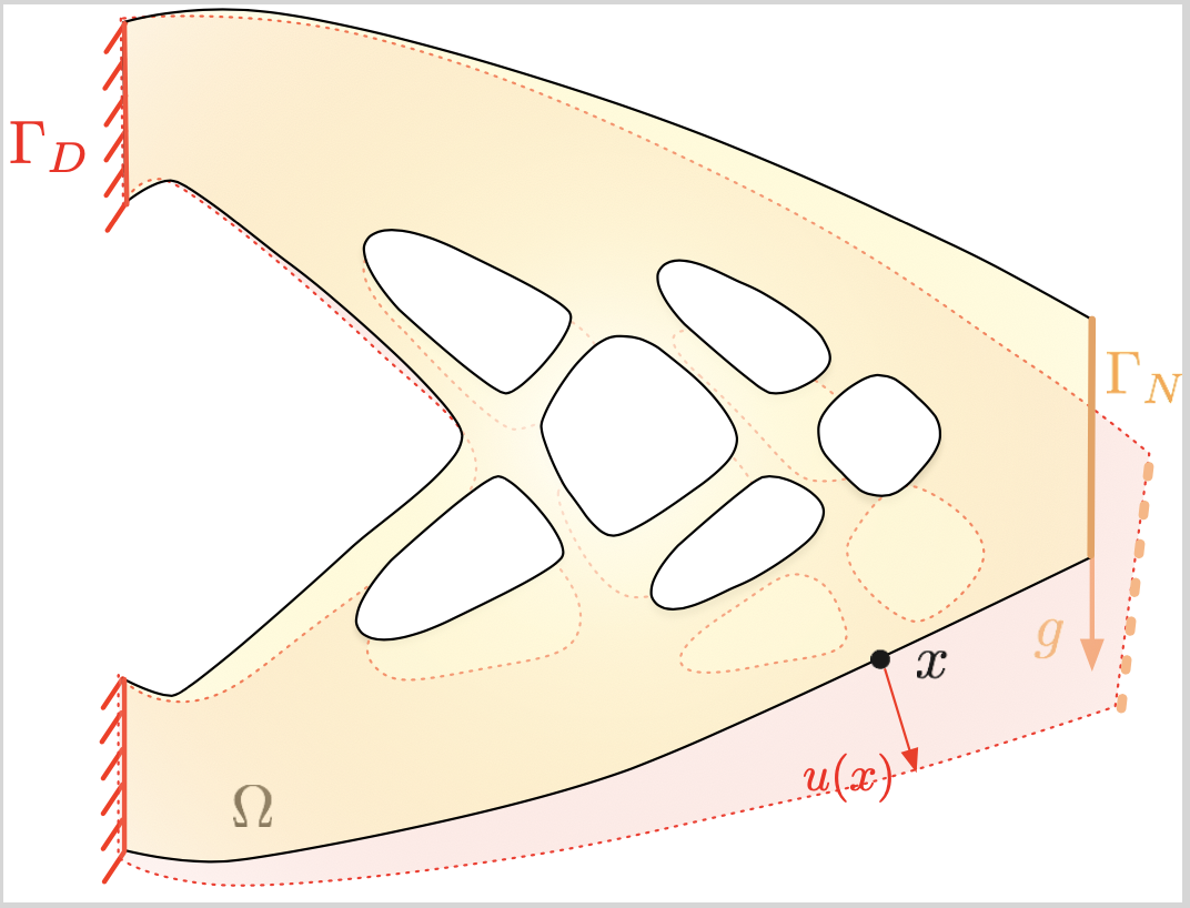
Fig. 3.1 The elastic structure \(\Omega\) realizes the displacement \(\u\) under the effect of body forces \(\textbf{f} : \Omega \to \mathbb{R}^d\) and surface loads \(\textbf{g} : \Gamma_N \to \mathbb{R}^d\).
In this section, we are interested with linear elasticity, where the displacement \(u\) and all its derivatives are assumed to be small, which allows for major simplifications in the mathematical equations.
The relative motion of the points of a structure \(\Omega\) undergoing a displacement \(\u\) is measured in terms of the linearized strain tensor \(e(\u) : \Omega \to \mathbb{R}^{d \times d}_{\text{\rm sym}}\), defined by:
For a point \(\x \in \Omega\), the physical interpretation of the matrix \(e(\u)(\x)\) is as follows, see Fig. 3.2 for an illustration:
For \(i=1,\ldots,d\), the diagonal entry \(e(u)(x)_{ii}\) encodes the stretching or the compression effect induced by \(u\) in the direction \(e_i\); the length \(h \ll 1\) of the small line segment with endpoints \(x\) and \(x + he_i\) becomes, after deformation:
\[\lvert x + he_i + u(x+he_i) - (x+u(x)) \lvert \approx h + h e(u)(x)_{ii} .\]For \(i,j=1,\ldots,d\), \(i\neq j\), \(e(u)(x)_{ij}\) measures the distortion of angles between the directions \(e_i\) and \(e_j\); more precisely,
\[e(u)(x)_{ij} = \frac{1}{2}(\kappa_1+ \kappa_2), \text{ where } \kappa_1 \approx \tan \kappa_1 \approx \frac{\partial u_2}{\partial x_1}, \text{ and } \kappa_2 \approx \tan \kappa_2 \approx \frac{\partial u_1}{\partial x_2}.\]
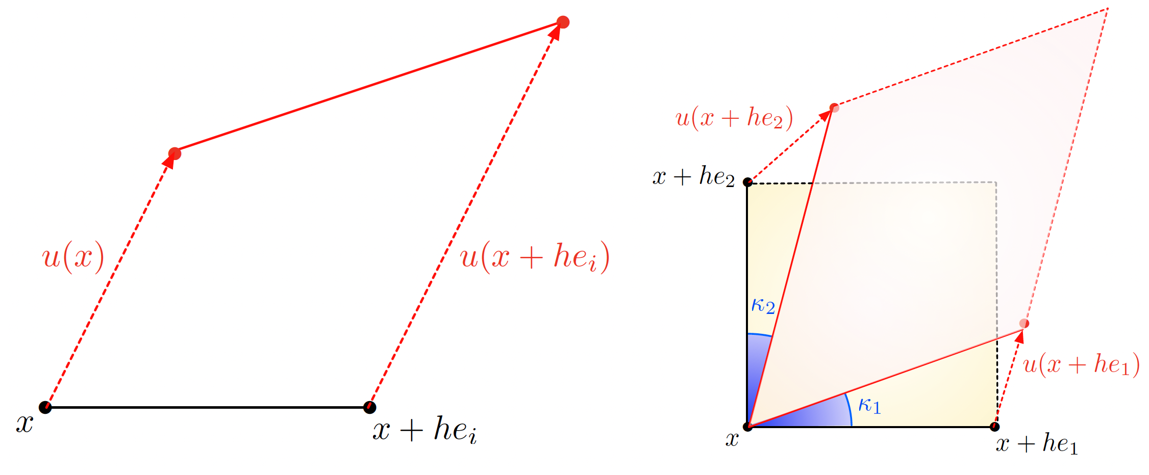
Fig. 3.2 Physical interpretation of the entries of the strain tensor \(e(u)(x)\); (a) The diagonal entry \(e(u)(x)_{ii}\) appraises the variation of the segment \([x,x+he_i]\) after deformation; (b) The off-diagonal entry \(e(u)(x)_{12}\) measures the variation of the angle between \([x,x+he_1]\) and \([x,x+he_2]\) after deformation.
Another means to appraise how \(e(u)\) accounts for the deformation of lengths and angles induced by \(u\) is the following. Let \([0,1] \ni t \mapsto \gamma(t)\) be a curve drawn within \(\Omega\), with length:
The deformed version of \(\gamma\) is the curve \([0,1] \ni t \mapsto (\text{Id} + u)( \gamma(t))\), whose length equals:
where \(C(u)\) is the right Cauchy-Green strain tensor defined by
The latter depends in a nonlinear way on \(u\), and it measures exactly the deformation of lengths incurred by the displacement \(u\). The linearized strain tensor \(e(u)\) is the linear part of the tensor \(\frac12(C(u)-\text{I})\). Considering \(e(u)\) in place of \(C(u)\) is the first source of linearity in the classical linear elasticity model; this simplification is called the geometric linearity assumption.
3.1.3. Stresses
The second ingredient in the description of an elastic structure \(\Omega\) is the representation of internal and external efforts, also called stresses.
3.1.3.1. Cauchy’s stress tensor
This task involves Cauchy’s stress tensor \(\sigma : \Omega \to \mathbb{R}^{d \times d}\): for any point \(x \in \Omega\) and any unit vector \(n \in \mathbb{S}^{d-1}\), \(\sigma(x) n\) is the force applied by the outer medium on the face of an infinitesimally small cube of material around \(x\), see Fig. 3.3. The entries of the tensor \(\sigma(x)\) can be separated between traction-compression entries and shear components, as depicted on Fig. 3.3 (b), (c):
For \(i=1,\ldots,d\), \(\sigma(x)_{ii}\) represents the \(i^{\text{th}}\) component of the force applied on the face oriented by \(e_i\); it thus accounts for a compression effect when \(\sigma(x)_{ii} < 0\), and a stretching (or dilation) effect if \(\sigma(x)_{ii} >0\).
For \(i,j=1,\ldots,d\), \(i\neq j\), the off-diagonal entry \(\sigma(x)_{ij}\) is the \(i^{\text{th}}\) component of the force applied on the face oriented by \(e_j\); it accounts for a shearing effect, whereby this face undergoes a tangential deformation.
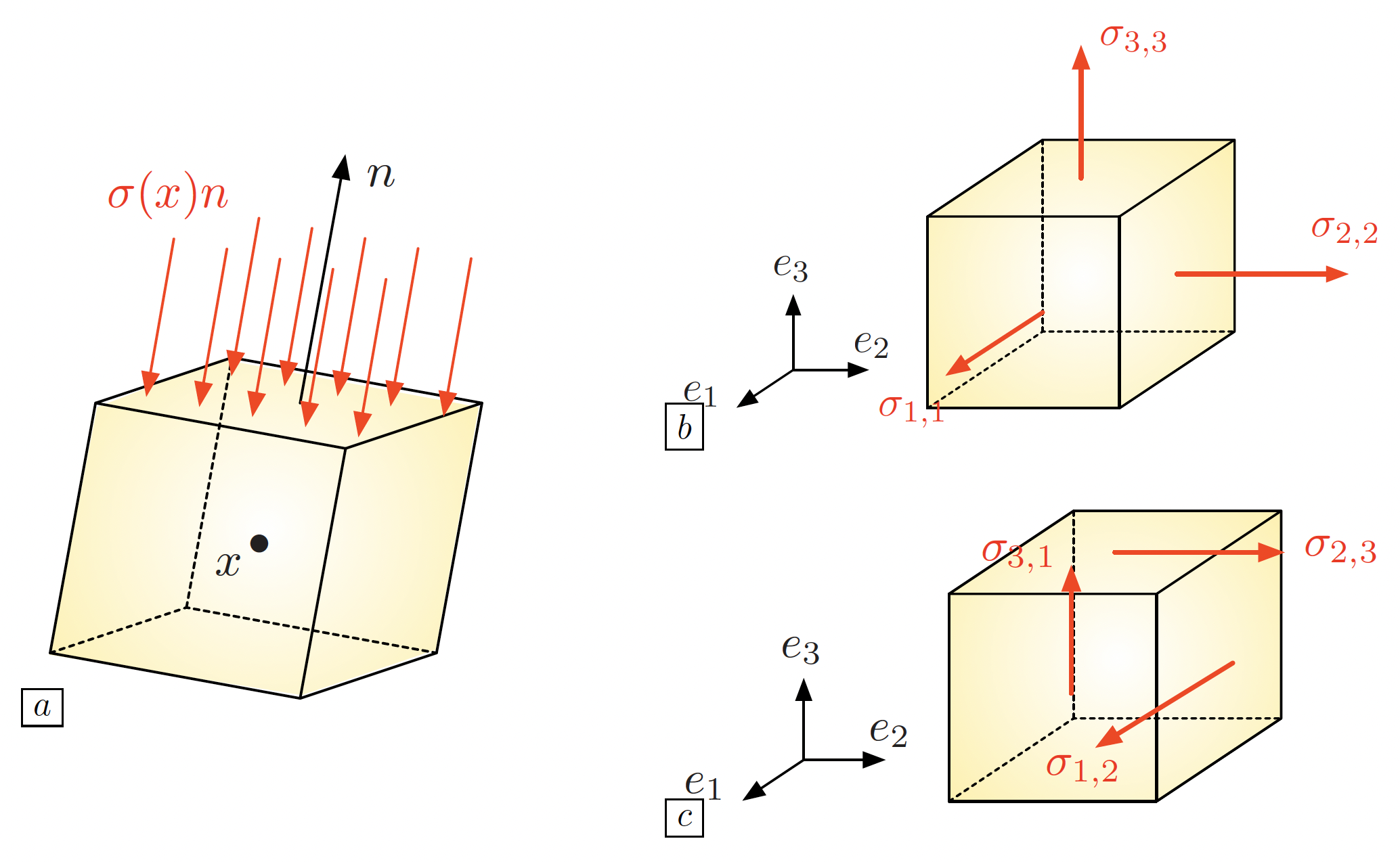
Fig. 3.3 The stress tensor: (a) For \(x\in \Omega\) and \(n \in \mathbb{S}^{d-1}\), the vector \(\sigma(x) n\) is the force imposed by the outer medium onto the face oriented by \(n\) of a small cube around \(x\); (b) The diagonal entries of \(\sigma(x)\) account for the compression efforts felt by this cube; (c) The off-diagonal entries encode the shear effects imposed on this cube.
Theorem 3.1
The stress is linear.
Proof
Cauchy’s tetrahedron
3.1.3.2. The laws of equilibrium
The stress tensor allows to express the conditions of equilibrium of a structure \(\Omega\). Let \(f: \Omega \to \R^d\) be the density of body forces (e.g. gravity) at play in \(\Omega\), and let \(g: \Gamma_N \to \R^d\) be the density of surface loads, applied on a fixed subset \(\Gamma_N\) of \(\partial \Omega\). Then:
The law of balance of linear momentum states that, for each subdomain \(\omega \Subset \Omega\), the sum of the body forces inside \(\omega\) and the forces applied by the rest of the structure on \(\partial \omega\) must vanish, i.e.
\[\int_\omega f \:\text{d} x + \int_{\partial \omega} \sigma n \:\text{d} s = 0.\]After application of the Green’s formula of cref{prop.Green}, this rewrites:
\[\int_\omega (\text{div}(\sigma) + f ) \:\text{d} x= 0,\]and since this relation should hold for any subdomain \(\omega \Subset \Omega\), it follows:
\[-\text{div}(\sigma) = f \text{ in } \Omega.\]Applying the same principle inside a small enough subdomain \(\omega \subset \Omega\) whose boundary contains a portion of \(\Gamma_N\), we obtain:
\[\int_\omega f \:\text{d} x + \int_{\partial \omega \cap \Gamma_N} g \:\text{d} s + \int_{\partial \omega \setminus \overline{\Gamma_N}} \sigma n \:\text{d} s = 0,\]that is:
\[\int_\omega f \:\text{d} x + \int_{\partial \omega} \sigma \cdot n \:\text{d} s + \int_{\partial \omega \cap \Gamma_N} g \:\text{d} s -\int_{\partial \omega \cap \Gamma_N} \sigma n \:\text{d} s = 0.\]Using Green’s formula on the second term in the above left-hand side together with the fact that \(-\text{div}(\sigma) = f\) inside \(\omega\), we obtain that the first two terms of the above equation vanish; since \(\omega\) is arbitrary, this entails:
\[\sigma n = g \text{ on } \Gamma_N.\]Note that this fact can also be understood as an application of the law of reciprocal actions.
One last consequence of equilibrium is that \(\Omega\) should be in rotational equilibrium. This implies the symmetry of the stress tensor, as expressed by the next result.
Theorem 3.2 (Cauchy’s theorem)
For any point \(x \in \Omega\), the tensor \(\sigma(x)\) is symmetric:
Proof
This is a non trivial consequence of the law of balance of momentum: no subdomain \(\omega \Subset \Omega\) should undergo rotational efforts induced by the outer medium.
3.1.4. Constitutive laws
The above description of an elastic structure is completed by a constitutive relation between the stress \(\sigma\) inside \(\Omega\) and the induced strain \(e(\u)\). In multiple applications, it is supposed to be linear, of the form:
Here, the a priori inhomogeneous (i.e. space dependent) tensor \(A\) and its inverse \(S\) are the Hooke’s tensor and the compliance tensor of the material, respectively. For \(\x \in \Omega\), \(A(\x)\) and \(S(\x)\) are linear mappings from \(\Rsym\) into itself, encoding the local properties of the constituent material of \(\Omega\) around \(x\), in a way which we now discuss more precisely. To this end, we focus on the three-dimensional context; the 2d case is evoked in remark 3.1. Also, to simplify the discussion, we assume the considered material to be homogeneous.
In general, \(A\) is a fourth-order tensor \(A = \left\{A_{ijkl} \right\}_{i,j,k,l=1,\ldots,3}\) with the following symmetries:
Hence, \(A\) has \(21\) independent entries. Fortunately, most materials present symmetries, which allows to reduce the number of these independent entries:
Isotropic materials exhibit the same behavior in all directions of space; their Hooke’s tensor \(A\) is completely characterized by two scalar parameters \(\lambda\) and \(\mu\), called the Lamé parameters of the material:
(3.1)¶\[\forall \xi \in \mathbb{R}_{\text{sym}}^{3\times 3} , \quad A\xi = 2\mu \xi + \lambda \tr(\xi) \I.\]The parameter \(\mu\) is called the shear modulus; it corresponds to the angular deviation caused by a unit shear stress, see Fig. 3.4 (a); the physical interpretation of \(\lambda\) is unfortunately not as clear. Usually, two more physical quantities \(E\) and \(\nu\) are used, from which \(\lambda\) and \(\mu\) can be retrieved as:
\[\mu = \frac{E}{2(1+\nu)}, \text{ and } \lambda = \frac{E\nu}{(1+\nu)(1-2\nu)}.\]The Young’s modulus \(E\) measures the resistance of the material to traction and compression, and the Poisson’s ratio \(\nu\) measures its resistance to transverse deformations, see Fig. 3.4 (b).
A more general class of materials is that of orthotropic materials. These possess three orthogonal planes of symmetry, and as a result, they enjoy different properties along the corresponding axes. They are characterized by one Young’s modulus \(E_i\) in each direction \(i=1,2,3\), one Poisson’s ratio \(\nu_{ij}\) and one shear modulus \(G_{ij}\) for each pair \(i\neq j\). One example of an orthotropic material is depicted on Fig. 3.5 (a).
Transversely isotropic materials have a particular form of orthotropy. They have one plane of symmetry, and show an isotropic behavior within any plane parallel to the latter. The physical properties of a material with transverse isotropy, say in direction \(e_3\), are characterized by five independent parameters: two Young’s moduli \(E_3\) and \(E_1 = E_2\) encoding the resistance to stretching in the transverse and longitudinal directions, respectively, two Poisson’s ratios \(\nu_{13} = \nu_{23}\) and \(\nu_{12}\) and the shear modulus \(G_{13} = G_{23}\) between the transverse and longitudinal directions. One example of a transversely isotropic material is depicted on Fig. 3.5 (b).
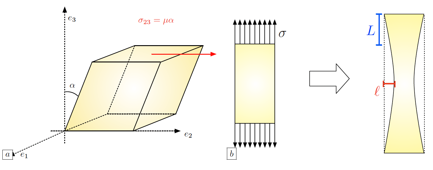
Fig. 3.4 Elastic parameters: (a) The shear modulus \(\mu\) accounts for the force \(\sigma_{23} = \mu \alpha\) that should be applied on the face oriented by \(e_3\) of a piece of material in the transverse direction \(e_2\) to create an angle \(\alpha\) with the \(e_3\) direction; (b) The Young’s modulus \(E = \sigma/L\) accounts for the amplitude of the force \(\sigma\) needed to stretch a piece of material by a length \(L\); the Poisson’s ratio \(\nu = -\ell / L\) measures the relative transverse displacement in this process.
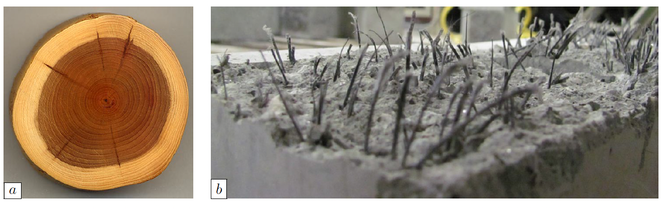
Fig. 3.5 Two different elastic materials: (a) Wood is an orthotropic material with large stiffness in the direction of the grain, low stiffness in the radial direction, and intermediate stiffness in the azimuthal direction; (b) Fiber-reinforced concrete is a transversely isotropic material: it is much stiffer in the direction of the metallic fibers than in the orthogonal directions.
Remark 3.1
The above considerations related to the elastic properties of structures take place in the physically prevalent setting of three space dimensions. The definition of the Hooke’s tensor \(A\) of a 2d structure depends on how the latter accounts for a 3d one which is invariant in the \(e_3\) direction. In plane stress, where the components \(\sigma_{i3} = \sigma_{3i}\) of the stress tensor vanish (\(i=1,2,3\)), the Lamé parameters \(\lambda\) and \(\mu\) characterizing the 2d tensor \(A\) in (3.1) are obtained from the Young’s modulus \(E\) and the Poisson’s ratio \(\nu\) of the 3d material via the relations:
\[\mu = \frac{E}{2(1+\nu)}, \text{ and } \lambda = \frac{E\nu}{1-\nu^2}.\]
In plane strain, where the components \(e(u)_{i3} = e(u)_{3i}\) of the strain tensor vanish, one has instead:
Remark 3.2
The strain tensor \(e(u)\) is by essence a Lagrangian quantity, as it is defined on the reference configuration \(\Omega\) of the structure. On the contrary, stresses are naturally expressed in the Eulerian variable, i.e. on the deformed configuration \((\text{Id} + u)(\Omega)\). Hence, the constitutive law should relate \(e(u)\) with a transported version of the stress tensor \(\sigma\) onto the reference configuration, called the Piola-Kirchoff stress tensor. In the present setting, this difficulty is ignored since both notions of stress tensors coincide at leading order, as the displacement of the structure is small, see the discussion in Chap. 13 of [TM05] about this point.
3.1.5. Boundary conditions
Clamping, traction, two-phase
3.1.6. Towards mathematical modeling: a typical boundary value problem
Gathering the concepts of the previous sections, we are in position to write down a prototype for boundary-value problems in the physical context of linearly elastic structures.
Let \(\Omega \subset \R^d\) be a structure which is attached on a region \(\Gamma_D\) of its boundary; it is submitted to body forces \(\textbf{f} : \Omega \to \R^d\) and surface loads \(\textbf{g} : \Gamma_N \to \R^d,\) applied on a region \(\Gamma_N\) of \(\partial \Omega\) disjoint from \(\Gamma_D\). The displacement \(\u\) of \(\Omega\) is the solution to the following system:
The mathematical framework associated to this system is similar to that presented in \cref{sec.1phaseconduc}. The Hooke’s tensor \(A : \Omega \to \calL(\Rsym,\Rsym)\) is a smooth enough mapping satisfying the following ellipticity property:
The body forces and surface loads \(f\) and \(g\) belong to the respective spaces \(L^2(\Omega)^d\) and \(L^2(\Gamma_N)^d\) and the displacement \(u\) is sought as the solution to the variational problem:
whose well-posedness follows from the Lax-Milgram theory – the coercivity of the involved bilinear form being a consequence of cref{eq.ellelas} and the Korn’s inequality, see for instance cite{ciarlet2021mathematical}.
Remark 3.3
The elliptic regularity theory, which loosely speaking ensures that, under suitable assumptions on \(\Omega\), \(f\) and \(g\), the solution \(u\) to \cref{eq.elas} is smooth, can be deployed pretty much as in the scalar case of the conductivity equation evoked in \cref{rem.ellregconduc}. As is exemplified in the sketch provided in \cref{sec.appellreg}, the pivotal ingredient of this theory is the ellipticity assumption \cref{eq.ellelas}, ensuring a control of the norm of \(u\) in terms of the operator \(\u \mapsto -\text{div}(Ae(\u))\).
3.1.7. Energy
Much intuition about the behavior of an elastic structure can be gleaned from energetic considerations. The fundamental result in this study is the following.
Theorem 3.3
Let the structure \(\Omega\) under scrutiny be in a deformed state characterized by the displacement \(u\). The work done by internal forces when this structure is further displaced by a small increment \(v\) equals:
Equivalently, in order to bring the structure from the configuration defined by \(u\) to that defined by \(u+v\), one has to supply an amount of energy equal to \(\int_\Omega \sigma(u) : e(v) \:\text{d} x\).
Proof
Bla bla
Note that, when \(v\) is of the form \(v = \text{d} h u\) with \(\text{d} h \ll 1\), the work (3.2) is negative, indicating that internal forces always work against the actual motion.
The total strain energy needed to bring \(\Omega\) from rest to \((\text{Id} + u)(\Omega)\) is obtained by integrating the above increment between both configurations, which reads:
Physically, the elastic energy of a system is the potential energy stored in the latter as the deformation occurs under the effect of work performed on it. This energy can then be converted and released under various forms, such as kinetic or thermal energy.
Likewise, when the structure is further deformed according to a small increment \(v\) from the deformed configuration characterized by \(u\), the work of external loads is
This quantity is positive when \(v\) is oriented in the direction of the forces \(f\) and \(g\): intuitively, these then work in favor of the motion by handing energy to the system. The total work of \(f\) and \(g\) when \(\Omega\) passes from rest to the deformed configuration \((\text{Id} + u)(\Omega)\) is obtained by a similar integration as above:
Finally, the total energy \(E(u)\) stored by \(\Omega\) in the displacement from rest to \((\text{Id} + u)(\Omega)\) equals:
The actual displacement \(u_\Omega\) of \(\Omega\), which we have characterized as the solution to \cref{eq.elas} in the previous section, is obtained by minimizing \(E(u)\) among all the possible displacements of the structure, that is:
The mathematical equivalence between \cref{eq.elas} and \cref{eq.minpot} follows from a classical application of the Lax-Milgram theory. Note that, using the variational problem \cref{eq.varfelas} satisfied by \(u_\Omega\), the minimum value of the energy \(E(u)\) reads:
This quantity is always nonpositive, reflecting that the application of external forces \(f\) and \(g\) to the structure \(\Omega\) always triggers a motion of the latter by conveying energy (which is thus subtracted from its potential energy).