2.5. The Level Set method: Part I

The topic in the spotlight of this section is the Level Set Method. In a nutshell, this general philosophy advocates to represent a domain implicitly to track its evolution in time.

This section is the first of a two-part discussion: basic facts are presented about implicit representations and operations based on the latter in Section 2.5.1 and Section 2.5.2; the development of fictitious domain methods for the resolution of boundary-value problems is then detailed in Section 2.5.3. The next Section 2.6 deals with more advanced features, and notably the treatment of evolving domain problems with the Level Set Method.

Before getting into the core of the matter, let us highlight a few useful references. The Level Set Method was introduced in the seminal article [OS88]; the comprehensive books [Set99] and [OF06] are very valuable complements to the succinct presentation of this tutorial. The reader might also find interest in the slides of a graduate course given by the author at Université Grenoble-Alpes.

2.5.1. Implicit representation

Let \(D\) be a bounded domain in \(\R^d\), where \(d=2\) or \(3\), containing the domain of interest \(\Omega \subset D\). The Level Set Method consists in looking to \(\Omega\) as the negative subset of a "Level Set function" \(\phi: D \to \R\), that is:

(2.7)\[\begin{split}\left\{\begin{array}{cl} \phi(\x) < 0 & \text{if } \x \in \Omega,\\ \phi(\x) = 0 & \text{if } \x \in \partial\Omega,\\ \phi(\x) > 0 & \text{otherwise.}\end{array}\right.\end{split}\]

This change of viewpoints is illustrated on Fig. 2.8.

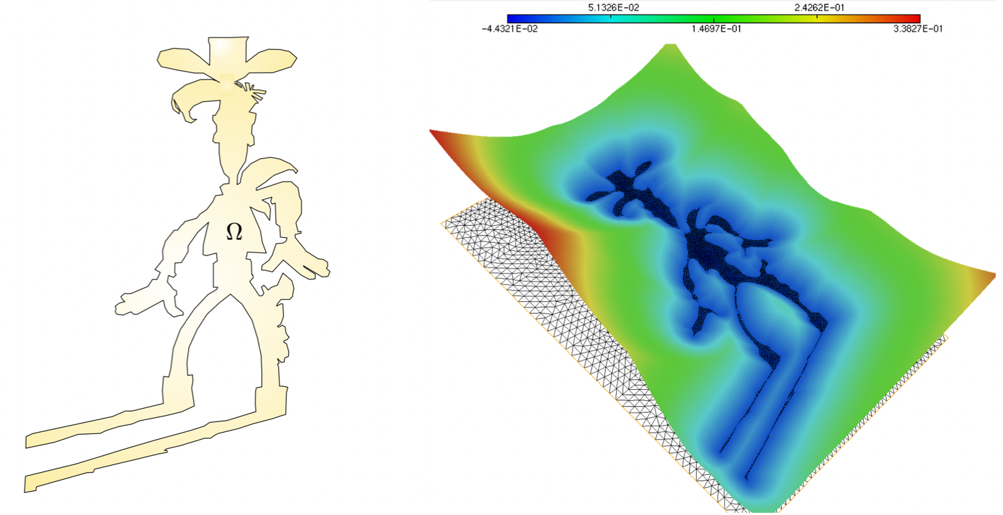
Fig. 2.8 (Left) One 2d domain \(\Omega\); (right) graph of an associated Level Set function \(\phi: D\to \R\).

2.5.2. Handling geometry with Level Set functions

One might fear that switching from a conventional to a Level Set representation of a domain entails a loss of information about its geometry. This is fortunately not the case, and we present below a few geometric operations that can be conveniently carried out from Level Set functions.

2.5.2.1. The normal vector

Let \(\Omega \subset \R^d\) be a smooth bounded domain, and let \(\phi : \R^d \to \R\) be an associated smooth Level Set function (i.e. (2.7) holds); we also assume that the gradient of \(\phi\) does not vanish in a neighborhood of \(\partial \Omega\).

The unit normal vector \(\n(\x)\) to \(\partial \Omega\) pointing outward \(\Omega\) is then expressed in terms of \(\phi\) as:

(2.8)\[\forall \x \in \partial \Omega, \quad \n(\x) = \frac{\nabla \phi(\x)}{\lvert \nabla\phi(\x)\lvert},\]

see Fig. 2.9 for an intuition.

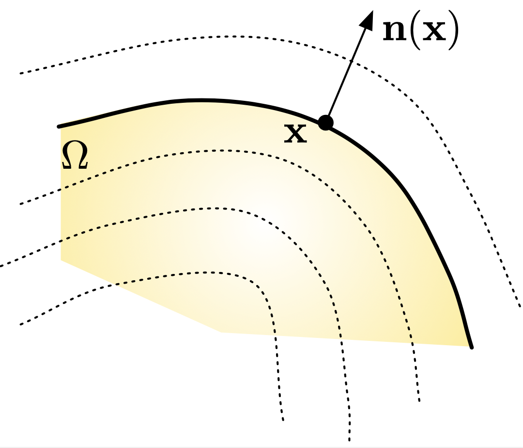
Fig. 2.9 The unit normal vector \(\n(\x)\) to \(\partial \Omega\) at \(\x \in \partial \Omega\) is the direction of largest variations of the values of \(\phi\) near \(\x\) (which is \(\nabla\phi(\x)\)); it is also orthogonal to the isosurfaces of \(\phi\).

Note that the above right-hand side is actually well-defined in the whole computational domain \(D\), at least at those points \(\x\) where \(\nabla \phi(\x)\) does not vanish, so that (2.8) actually accounts for an extension of the unit normal vector \(\n\) to \(D\).

2.5.2.2. The mean curvature

In the same context as in the previous section, the mean curvature of \(\partial\Omega\) can be calculated from the (admitted) following formula:

(2.9)\[\forall \x \in \partial \Omega, \quad \kappa(\x) = \dv \left(\frac{\nabla \phi}{\lvert\nabla \phi \lvert} \right)(\x).\]

Like the formula (2.8) for \(\n(\x)\), this expression actually accounts for a natural extension of the mean curvature away from the boundary \(\partial \Omega\).

2.5.2.3. Operations on sets

Let \(\Omega\), \(\Omega_1\), \(\Omega_2\) be bounded domains in \(\R^d\), and let \(\phi\), \(\phi_1, \phi_2: \R^d \to \R\) be associated Level Set functions. Then,

• One Level Set function \(\phi_c\) for the complement \(^{c}\overline{\Omega}\) of \(\Omega\) is:

  \[\phi_c =- \phi.\]

• One Level Set function \(\phi_u\) for the reunion \(\Omega_1 \cup \Omega_2\) is:

  \[\phi_u = \min(\phi_1,\phi_2).\]

• One Level Set function \(\phi_i\) for the intersection \(\Omega_1 \cap \Omega_2\) is:

  \[\phi_i = \max(\phi_1,\phi_2).\]

An illustration of the second formula is given in Fig. 2.10.

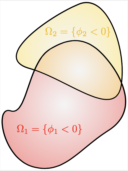
Fig. 2.10 One Level Set function \(\phi_u\) for the reunion of \(\Omega_1\), \(\Omega_2\) is the minimum of Level Set functions \(\phi_1\), \(\phi_2\) for \(\Omega_1\), \(\Omega_2\).

2.5.2.4. Calculation of normal vectors and mean curvatures with Level Set functions in \(\texttt{FreeFem}\)

In this section, we discuss how the formulas introduced in Section 2.5.2.1 and Section 2.5.2.2 allow to calculate the normal vector and the mean curvature of the boundary of a domain \(\Omega\) when the latter is only supplied via a Level Set function. The code associated to this section is contained in here

Let \(\Omega \subset \R^2\) be a smooth bounded domain, contained in a larger computational domain \(D\). Let \(\calT\) be a mesh of \(D\), and let \(\phi : \R^2 \to \R\) be a Level Set function for \(\Omega\), discretized as a \(\P_1\) Finite Element function on \(\calT\).

Let us first consider the practical calculation of the normal vector \(\n: \partial \Omega \to \R^2\). The formula (2.8) can be used readily to this end, as in the following listing.

/* Calculation of the components (nx,ny) of the normal vector field n = \frac{\nabla\phi}{\lvert\nabla\phi\lvert} as P0 functions */
norm0 = sqrt( dx(phi)^2 + dy(phi)^2 + EPS );
nx0 = dx(phi) / norm0;
ny0 = dy(phi) / norm0;

Since \(\phi\) is a \(\P_1\) Finite Element function, the normal vector is naturally calculated as a (discontinuous) \(\P_0\) function, and it is often desirable to handle a \(\P_1\) vector field. To achieve this, we rely on a useful general trick to reconstruct a \(\P_1\) Finite Element function \(u\) from a \(\P_0\) function \(u_0\). We solve the following variational problem:

\[\text{Search for } u \in H^1(D) \text{ s.t. } \forall v \in H^1(D), \quad \alpha^2 \int_\Omega \nabla u \cdot \nabla v \:\d \x + \int_\Omega uv \:\d \x = \int_\Omega u_0 v \:\d \x,\]

by choosing the space of \(\P_1\) Finite Elements for the discretization of \(H^1(D)\). Here, the first integral in the above left-hand side is the bilinear form associated to the Laplace operator, weighted by the "small" parameter \(\alpha\) (often chosen of the order of the mesh size). It allows to additionally smooth the input field \(u_0\) over a length-scale \(\alpha\) by virtue of the regularizing properties of this operator, as a means to eliminate undesirable numerical artifacts. This procedure is implemented in the following listing.

/* Reconstruction of a P1 vector field for the normal vector;
   Add a small smoothing with the Laplacian term \alpha^2 \Delta u */
problem normalx(nx,v) = int2d(Th)( alpha^2*(dx(nx)*dx(v)+dy(nx)*dy(v)) + nx*v )
                        - int2d(Th)( nx0*v);

problem normaly(ny,v) = int2d(Th)( alpha^2*(dx(ny)*dx(v)+dy(ny)*dy(v)) + ny*v )
                        - int2d(Th)( ny0*v);

normalx;
normaly;

norm1 = sqrt( nx^2 + ny^2 + EPS );
nx = nx / norm1;
ny = ny / norm1;

Let us now turn to the mean curvature \(\kappa\). Judging from (2.9), it is tempting to calculate the extended normal vector \(\n = \frac{\nabla \phi}{\lvert \nabla \phi \lvert}\) as a \(\P_0\) function on \(\calT\), to reconstruct a \(\P_1\) function on \(\calT\) by a similar trick as in the previous listing, and then to take derivatives in the result. Unfortunately, the successive differentiation and \(\P_1\) reconstructions of this strategy are likely to cause numerical instabilities.

In order to alleviate the need for reconstructing \(\P_1\) Finite Element functions, we rely on the following application of the Green’s formula:

\[\forall v \in H^1(D), \quad \int_D \kappa v \:\d \x = \int_{\partial D} (\n\cdot \n_D) v \:\d s - \int_D \n \cdot \nabla v\:\d \x,\]

where \(\n = \frac{\nabla \phi}{\lvert \nabla \phi\lvert}\) is the (extended) normal vector to \(\partial \Omega\) and \(\n_D\) is the unit normal vector to \(\partial D\). Now, in order to calculate \(\kappa\), we directly solve the following variational problem:

\[\text{Search for } u \in H^1(D) \text{ s.t. } \forall v \in H^1(D),\quad \int_D \alpha^2 \nabla u \cdot \nabla v \:\d\x + \int_D uv \:\d \x = -\int_D \n \cdot \nabla v\:\d \x + \int_{\partial D} (\n\cdot \n_D) v \:\d s.\]

2.5.3. Application: fictitious domain methods

Sometimes in realistic applications, it may be very complicated to obtain a mesh of the considered domain \(\Omega\). It is often easier to introduce a larger, "simple" computational domain \(D\) (e.g. a box), for which it is possible to construct a mesh \({\mathcal T}\). The domain \(\Omega\) is not meshed, but efficient methods (such as those broached in the next Section 2.6.1) allow to generate an associated level set function \(\phi : D \to \R\). An illustration of this situation is provided in Fig. 2.11.

In such a setting where it is difficult to directly apply the methods of Section 1.4 for the resolution of boundary value problems on \(\Omega\), a fictitious domain method ca be used. Essentially, an approximate problem is introduced, parametrized by a "small" parameter \(\varepsilon \ll 1\), which is posed on the larger domain \(D\). It gives rise to a solution \(u_\varepsilon : D \to \R\) whose restriction to \(\Omega\) is expected to be close to that of the original model: \(u_\varepsilon \lvert_\Omega \approx u\).

Understandably enough, the definition of this approximate problem depends on the nature of the original one, and to illustrate this practice, we consider two model situations.

Let \(\Omega\) be the domain depicted on Fig. 2.11, (left), a mesh of which is supplied here. We consider the following boundary-value problems:

(2.10)\[\begin{split}\left\{ \begin{array}{cl} - \Delta u_1 = 0 & \text{in } \Omega, \\ u_1 = u_D & \text{on } \Gamma_D, \\ \frac{\partial u_1}{\partial n} = g & \text{on } \Gamma_N, \\ \frac{\partial u_1}{\partial n} = 0 & \text{on } \Gamma, \end{array} \right. \:\:\text{ and }\:\: \left\{ \begin{array}{cl} - \Delta u_2 = 0 & \text{in } \Omega, \\ u_2 = u_D & \text{on } \Gamma_D, \\ \frac{\partial u_2}{\partial n} = g & \text{on } \Gamma_N, \\ u_2= 0 & \text{on } \Gamma. \end{array} \right.\end{split}\]

Both problems differ only by the type of boundary conditions imposed on the region \(\Gamma\) of \(\partial \Omega\). The code associated to their resolution is available here, see Fig. 2.12 (left) and Fig. 2.13 (left) for the results.

We now consider the situation where no mesh of \(\Omega\) is available. Instead, a mesh \(\calT\) of a larger computational box \(D\) is provided (which can be downloaded here), together with a Level Set function \(\phi : D \to \R\) for \(\Omega\) (click here), see Fig. 2.11 (middle,right).

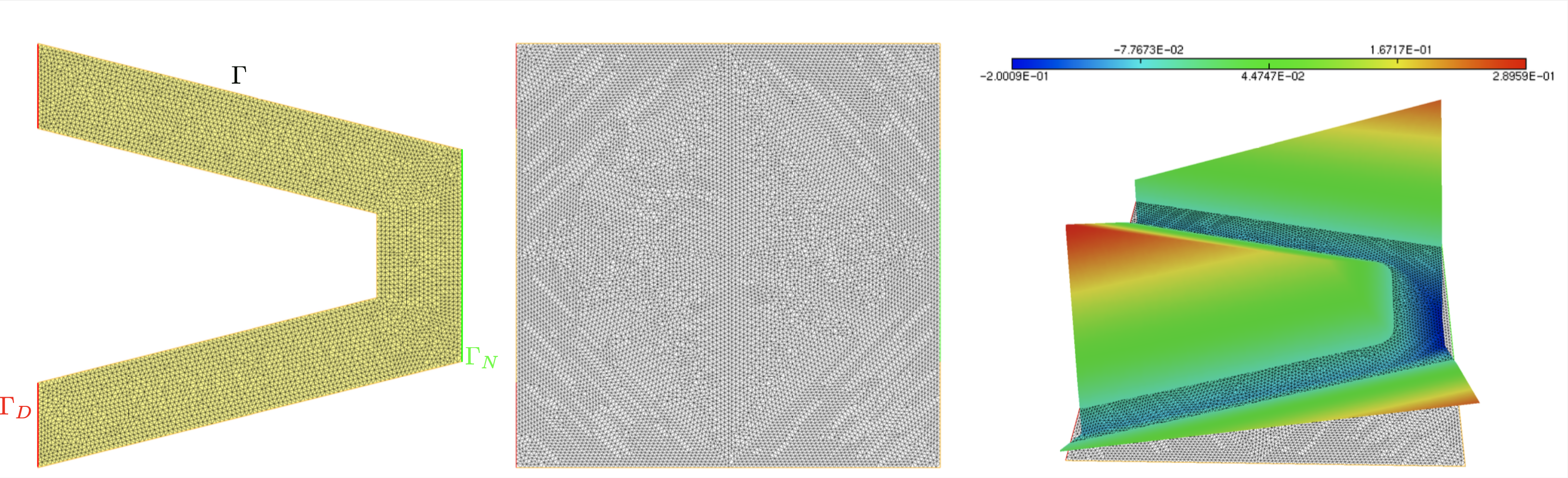
Fig. 2.11 (Left) The considered domain \(\Omega\); (middle) Mesh of the large computational box \(D\); (right) Graph of a Level Set function \(\phi: D\to \R\) for \(\Omega\).

The next two exercises analyze how to approximately solve both problems (2.10) in this context. The code for both examples is contained in this file, and the numerical results are represented in Fig. 2.12 and Fig. 2.13.

Exercise (Computation of \(u_1\) by the ersatz material method)

Let \(u_{1,\e}\) be the unique solution in \(H^1(D)\) to the following boundary-value problem:

(2.11)\[\begin{split} \left\{\begin{array}{cl} -\dv(\gamma_\varepsilon(\x) \nabla u _{1,\varepsilon} ) = 0 &\text{in } D, \\ u _{1,\varepsilon} = u_D & \text{on } \Gamma_D, \\ \frac{\partial u _{1,\varepsilon}}{\partial n} = g & \text{on } \Gamma_N, \\ \frac{\partial u _{1,\varepsilon}}{\partial n} = 0 & \text{on } \partial D \setminus (\overline{\Gamma_D} \cup \overline{\Gamma_N}). \end{array} \right.\end{split}\]

Here, the conductivity \(\gamma_\varepsilon(x)\) equals \(1\) if the point \(x\) is "well-inside" \(\Omega\) and a very low value \(\varepsilon\) if it is "well-outside" \(\Omega\). In a thin band around \(\partial \Omega\), it interpolates between these two values. One possible definition of \(\gamma_\e\) exhibiting this behavior is:

\[\gamma_\varepsilon(\x) = \max\left(\varepsilon, \frac{1}{2}\left(1+\tanh\left(-\frac{\phi(\x)}{\varepsilon} \right)\right) \right), \quad \x \in D.\]

Solve (2.11) with \(\texttt{FreeFem}\) and compare its solution \(u_{1,\e}\) to that \(u_1\) of (2.10) (left).

(Remark: An argument similar to the proof of the exercise in Section 1.8 allows to prove that \(u_{1,\e} \to u_1\) in \(H^1(\Omega)\).)

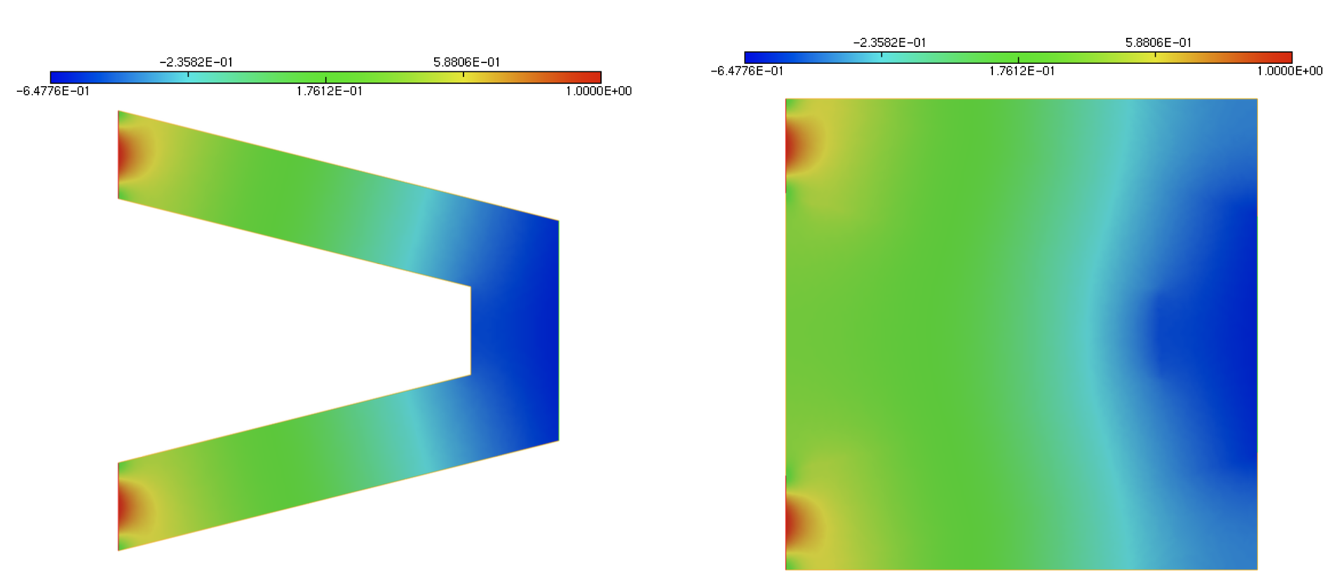
Fig. 2.12 (Left) Solution \(u_1\) of the Laplace equation on \(\Omega\) with homogeneous Neumann boundary conditions on \(\Gamma\); (right) Solution \(u_{1,\e}\) of the penalized version on the whole domain \(D\).

Exercise (Computation of \(u_2\) via the porosity method)

Let \(u_{2,\e}\) be the unique \(H^1(D)\) solution to the following boundary-value problem:

(2.12)\[\begin{split}\left\{ \begin{array}{cl} -\dv((1+c_\varepsilon(\x)) \nabla u _{2,\varepsilon} ) + c_\varepsilon(\x) u _{2,\varepsilon} = 0 &\text{in } D, \\ u _{2,\varepsilon} = u_D & \text{on } \Gamma_D, \\ \frac{\partial u _{2,\varepsilon}}{\partial n} = g & \text{on } \Gamma_N, \\ u _{2,\varepsilon} = 0 & \text{on } \partial D \setminus (\overline{\Gamma_D} \cup \overline{\Gamma_N}). \end{array} \right.\end{split}\]

Here, \(c_\varepsilon(\x)\) equals \(0\) if the point \(\x\) is "well-inside" \(\Omega\) and takes a very large value \(\frac{1}{\e}\) if it is "well-outside" \(\Omega\). In a thin band around \(\partial \Omega\), it interpolates between these two values. An example of a function showing this behavior is:

\[c_\varepsilon(\x) = \frac{1}{2\varepsilon}\left(1+\tanh\left(\frac{\phi(\x)}{\varepsilon}\right)\right), \quad \x \in D.\]

Solve (2.12) with \(\texttt{FreeFem}\) and compare its solution \(u_{2,\e}\) to that \(u_2\) of (2.10) (right).

(Remark: Again, it is possible to prove that \(u_{2,\e} \to u_2\) in \(H^1(\Omega)\).)

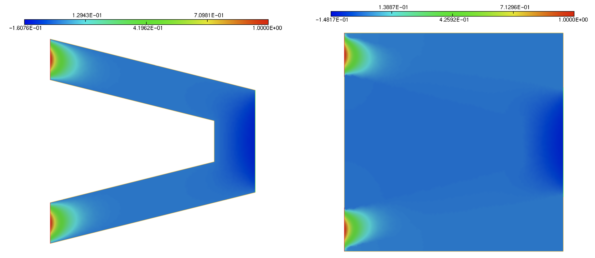
Fig. 2.13 (Left) Solution \(u_2\) of the Laplace equation on \(\Omega\) with Dirichlet boundary conditions on \(\Gamma\); (right) Solution \(u_{2,\e}\) of its penalized version on the whole domain \(D\).