2.1. Creating a mesh from an image

Throughout the situations considered in Section 1, the computational domain \(\Omega\) was generally simple enough (e.g. a mesh, a rectangle, …) so that it could be meshed from a parametrization of its boundary, as presented in Section 1.4.2. In many instances however, it is relevant to work with domains that are more peculiar. In this perspective, this section discusses a method for constructing a mesh from the input of a black-and-white image of a 2d domain \(\Omega\).

The complete script of the proposed method can be downloaded here and we comment about its most salient features below.

The procedure hinges on convenient built-in commands in \(\texttt{FreeFem}\). These work on images under the \(\texttt{.pgm}\) format; since images are usually rather supplied as \(\texttt{.jpg}\) files, we first use a conversion program in command line. This tool is part of the open-source library ImageMagick , which should be installed before running the script below.

/* Create a mesh from the datum of a black-and-white image (in jpg)
 !!!! The command line "convert" from ImageMagick must be available !!!! */
load "ppm2rnm"
load "isoline"
load "medit"

/* Decide whether to mesh the image (1) or its complement (0) */
int mshimg = 0;

/* Convert input image into pgm format */
string INPUT      = "obs.jpg";
string INPUTPGM   = "obs.pgm";
string OUTPUT     = "obs.mesh";

exec("convert "+INPUT+" "+INPUTPGM);

The next sequence of instructions reads the image as a 2d array of pixels; it creates a mesh \(\calT_h\) adjusted to the size of this array, and defines a \(\P_1\) Finite Element function, whose values at its vertices are the intensity values of the image – ranging from \(0\) (for black) to \(1\) (for white).

/* Read image and get data */
real[int,int] img(INPUTPGM);
int nx = img.n;
int ny = img.m;

/* Creation of a square mesh adapted to the pixellisation of the image */
mesh Th = square(nx-1,ny-1,[(nx-1)*(x),(ny-1)*(1-y)]);
fespace Vh(Th,P1);
Vh u;
u[] = img;

The \(\texttt{FreeFem}\) function isoline then allows to extract the \(0.5\) isoline of the image Finite Element function \(\texttt{u}\) as a collection of parametrized curves.

/* Extraction of the 0.5 isoline */
real[int,int] ver(3,1); // Table for the vertices of the isoline (will be resized automatically)
int[int] be(1); // Table for the beginning and end of each curve portion (will be resized automatically)
real thres = 0.5;

int nc = isoline(Th,u,iso=thres,close=1,ver,beginend=be,smoothing=0.1);

/* Endpoints of the longest isoline */
int ip0 = be(0);
int ip1 = be(1)-1;
int npc = 200; // Desired number of vertices on the boundary
int npb = 50; // Desired number of vertices on the outer border

/* Parametrization of the border from the datum of the boundary points */
border BIso(t=0,1) {P=Curve(ver,ip0,ip1,t); label=10; }
/* border left(t=0,1) {x=0.0; y=ny-ny*t; label=0; }
border bot(t=0,1) {x=nx*t; y=0.0; label=0; }
border right(t=0,1) {x=nx; y=ny*t; label=0; }
border top(t=0,1) {x=nx-nx*t; y=ny; label=0; }*/
border left(t=0,3) {x=-0.5*nx; y=2*ny-ny*t; label=1; }
border bot(t=0,2) {x=-0.5*nx+nx*t; y=-ny; label=0; }
border right(t=0,3) {x=1.5*nx; y=-ny+ny*t; label=2; }
border top(t=0,2) {x=1.5*nx-nx*t; y=2*ny; label=0; }

We eventually create the mesh of the image (or that of its complement) from the above set of boundary curves.

/* Creation of the mesh */
mesh Thfig;
if ( mshimg )
  Thfig = buildmesh(BIso(-npc));
else
  Thfig = buildmesh(left(npb)+bot(npb)+right(npb)+top(npb)+BIso(npc));

/* Scaling Thfig between 0 and 1 */
real[int] bb(4);
boundingbox(Thfig,bb); // bb[0] = xmin, bb[1] = xmax, bb[2] = ymin, bb[3] = ymax

real[int] gc = [0.5*(bb[0]+bb[1]),0.5*(bb[2]+bb[3])];
real dd = max(bb[1]-bb[0],bb[3]-bb[2]);
dd = 1.0/dd;

Thfig = movemesh(Thfig,[dd*(x-gc[0]),dd*(y-gc[1])]);

/* Save mesh */
savemesh(Thfig,OUTPUT);

An example, using this image is depicted in Fig. 2.1.

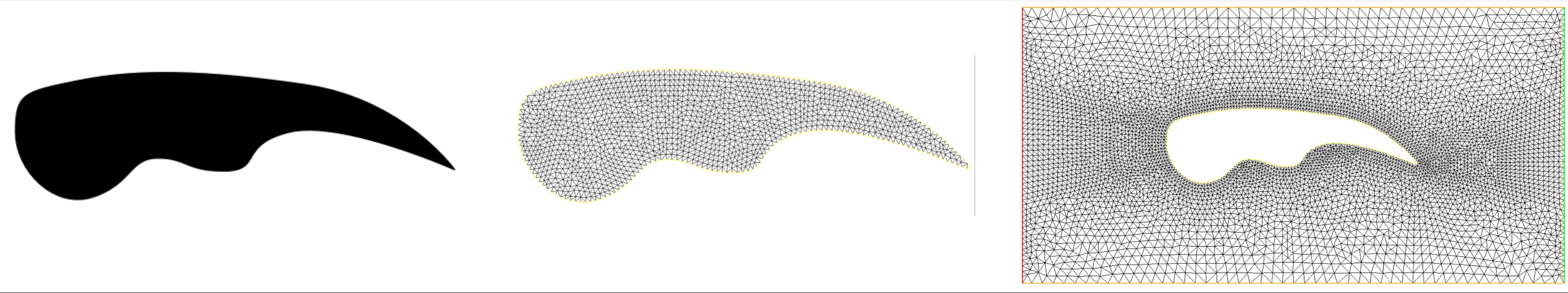
Fig. 2.1 (Left) A 2d domain \(\Omega\) supplied as a black-and-white picture (\(\texttt{.jpg}\) format); (middle) Mesh of \(\Omega\); (right) Mesh of the complement of \(\Omega\) within a box.