1.7. Eigenvalue problems

In this section, we consider the treatment of eigenvalue problems with \(\texttt{FreeFem}\). Beyond its physical relevance and ubiquity in applications, this task is a good opportunity to learn how to handle the Finite Element matrices involved in variational formulations.

1.7.1. Handling Finite Element matrices

Since Section 1.4, we have been solving variational problems with \(\texttt{FreeFem}\) via the keyword problem. This practice conveniently conceals the operations involved in the numerical resolution, notably the assembly and inversion of the stiffness matrix. This section describes an alternative way to solve a variational problem with \(\texttt{FreeFem}\) which is more intrusive, but also more flexible; the source code corresponding to this presentation can be downloaded here.

To set ideas, let us consider again the Laplace equation in an L-shaped domain \(\Omega\), introduced in Section 1.4: we look for the solution \(u \in H^1_0(\Omega)\) to the following boundary-value problem:

\[\begin{split}\left\{ \begin{array}{cl} -\Delta u = f & \text{in } \Omega, \\ u = 0 & \text{on } \partial \Omega, \end{array} \right. \quad \text{ where } f = 1.\end{split}\]

As we have seen, the variational formulation for this problem reads:

(1.27)\[\text{Search for } u \in H^1_0(\Omega) \text{ s.t. } \forall v \in H^1_0(\Omega), \quad \int_\Omega \nabla u\cdot \nabla v \:\d \x = \int_\Omega fv\:\d \x,\]

which becomes, after Finite Element discretization:

(1.28)\[\text{Search for the coefficient vector } \bU_h \in \mathbb{R}^{N_{V_h}} \:\: \text{ s.t. } \:\: K_h \bU_h = \bF_h,\]

where \(K_h\) is the \(N_{V_h} \times N_{V_h}\) stiffness matrix, and \(\bF_h \in\mathbb{R}^{N_{V_h}}\) is the force vector.

The main components of such a variational problem – i.e. its bilinear form and its right-hand side – may be entered in \(\texttt{FreeFem}\) thanks to the keyword varf, as in the following listing.

/* Finite Element spaces and functions */
fespace Vh(Th,P1);
Vh uh;

/* Variational formulation of the Laplace equation */
varf varlap(u,v) = int2d(Th)(dx(u)*dx(v)+dy(u)*dy(v))
                 + int2d(Th)(f()*v)   // Watch out for the sign!
                 + on(1,u=0);

Note that the sign between the bilinear and linear parts differs between this syntax and that attached to the keyword problem; this is because the present encoding does not allow to solve directly the variational problem. The stiffness matrix \(K_h\) and the force vector \(\bF_h\) of the Finite Element discretization (1.28) are constructed as follows.

/* Assembly of the stiffness matrix */
matrix A;
A = varlap(Vh,Vh,solver=UMFPACK);

/* Assembly of the right-hand side */
Vh rhs;
rhs[] = varlap(0,Vh); // rhs[] is the array with size
                    //the number of dofs of the Finite Element
                   // space, whose entries are the coefficients of rhs.

Here, we recall from remark 1.11 that the array containing the coefficients of a Finite Element function \(u\) is obtained by the command \(\texttt{u[]}\).

Finally, the Finite Element system (1.28) is inverted by the following natural command:

/* Resolution of the Finite Element system */
uh[] = A^-1 *rhs[];

1.7.2. An eigenvalue problem

Let \(\Omega\) be a bounded domain in \(\mathbb{R}^2\); we consider the following eigenvalue problem:

(1.29)\[\begin{split} \text{Search for } \lambda \in \mathbb{R} \text{ and } u \in H^1_0(\Omega), \: u\neq 0,\:\: \text{ s.t. } \left\{ \begin{array}{cl} -\Delta u = \lambda u & \text{in } \Omega, \\ u=0 & \text{on } \partial\Omega. \end{array} \right.\end{split}\]

Obviously, for any real value \(\lambda\), \(u = 0\) is solution to this problem. The sought eigenvalues are precisely those values \(\lambda\) for which a non trivial eigenfunction exists. It can actually be proved that these eigenvalues form a sequence of positive real numbers going to infinity:

\[0\leq \lambda_1 \leq \lambda_2 \leq ... \: \to \: \infty;\]

The peculiar property of eigenvalues is at the core of the modeling of multiple physical phenomena. For instance,

• When \(\Omega\) represents an elastic membrane, the values \(\lambda_n\) are its self-vibration frequencies;

• When \(\Omega\) is a thermal cavity, one may prove that the solution to the unsteady heat equation (1.25) decays exponentially fast in time, at the rate \(e^{-\lambda_1 t}\); the asymptotic profile of the temperature is then given by the first eigenvector \(u_1\).

In this tutorial, we shall not say much about the difficult, but fascinating spectral theory, dealing with the eigenelements of boundary-value problems, and we shall only formally describe their numerical calculation. We refer for instance to [All07] for a glimpse of the rigorous framework.

The resolution of (1.29) relies on a variational formulation, similar to that of a classical boundary-value problem, and we briefly rephrase the argument. Since the sought function \(u\) satisfies homogeneous Dirichlet boundary conditions, it is natural to work with the functional space \(V = H^1_0(\Omega)\), defined in Section 1.1.3.4.1. Multiplying the main equation of (1.29) by an arbitrary test function \(v \in H^1_0(\Omega)\) and using Green’s formula, we are led to the following problem:

\[\text{Search for } \lambda \in \R \text{ and } u \in V \text{ with } u \neq 0 \:\: \text{ s.t. } \:\: \forall v \in H^1_0(\Omega), \:\: a(u,v) = \lambda m(u,v).\]

This formulation brings into play the same continuous and coercive bilinear form \(a : V \times V \to \R\) as that involved in the variational problem for the Laplace equation, see Section 1.2, and an additional continuous, bilinear form \(m: V \times V \to \R\):

\[a(u,v) = \int_\Omega \nabla u \cdot \nabla v \:\d \x , \:\: \text{ and } \:\: m(u,v) = \int_\Omega uv \:\d \x.\]

Proceeding along the lines of Section 1.3, we now introduce a finite-dimensional subspace \(V_h\) of \(H^1_0(\Omega)\), we are led to the following Finite Element problem:

(1.30)\[\text{Search for } \lambda_h \in \R \text{ and } u_h \in V_h \text{ with } u_h \neq 0 \:\: \text{ s.t. } \:\: \forall v_h \in V_h, \:\: a(u_h,v_h)= \lambda_h m(u_h,v_h).\]

Let us now select a basis \(\left\{ \varphi_j\right\}_{j=1,...,N_h}\) of functions for \(V_h\); we denote by \(\bU_h = \left( u_j \right)_{j=1,...,N_h} \in \R^{N_h}\) the vector of the components of the sought eigenfunction \(u_h\) in this basis:

\[u_h = \sum\limits_{j=1}^{N_h}{u_j\varphi_j}.\]

Injecting this expression into the Finite Element problem (1.30) and taking test functions \(v_h = \varphi _i\), \(i=1,...,N_h\), we arrive at the following \(N_h \times N_h\) linear system:

\[K_h \bU_h = \lambda_h B_h \bU_h,\]

where the matrix \(K_h\) is the usual stiffness matrix for the Laplace equation, and \(B_h\) is the so-called mass matrix:

\[(K_h)_{ij} = \int_\Omega{\nabla \varphi_j \cdot \nabla \varphi_i \:\d\x}, \text{ and } (B_h){ij} = \int_\Omega{\varphi_j \varphi_i \:\d\x}.\]

We therefore end up with a generalized matrix eigenvalue problem, which can be conveniently solved thanks to the EigenValue command in \(\texttt{FreeFem}\).

The archetypal resolution of such an eigenvalue problem with \(\texttt{FreeFem}\) is exemplified in the following listing, where we use the syntax elements introduced in Section 1.7.1 to define the stiffness and mass matrices of the problem. The complete code can be downloaded here.

/* Variational formulations for the stiffness and mass matrices;
   the homogeneous Dirichlet b.c. has to be put only on the stiffness matrix */
varf stiffness(u,v) = int2d(Th)(dx(u)*dx(v)+dy(u)*dy(v)) + on(0,u=0.0);

varf mass(u,v) = int2d(Th)(u*v);

/* Getting matrices */
matrix A = stiffness(Vh,Vh,solver=CG);
matrix B = mass(Vh,Vh,solver=CG);

/* Setting parameters */
int nev = 20; // Number of computed eigenvalues
real[int] ev(nev); // Table of the computed eigenvalues
Vh[int] eV(nev); // Table for the eigenvectors
real sigma = 0.0; // Value around which the eigenvalues are computed.

/* Solving matrix eigenvalue problem */
int k = EigenValue(A,B,sym=true,sigma=sigma,value=ev,vector=eV,tol=1e-10,maxit=0,ncv=0);

The result of this procedure is depicted on Fig. 1.23.

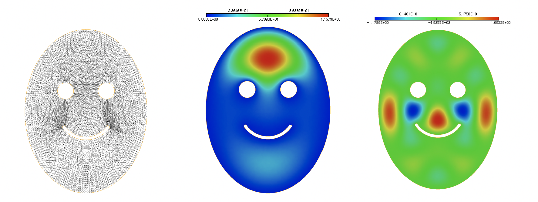
Fig. 1.23 (Left) Physical domain \(\Omega\) of the eigenvalue problem; (middle) Eigenfunction \(u_1\) associated to the first eigenvalue \(\lambda_1 \approx 7.61\); (right) Eigenfunction \(u_{20}\) associated to the \(20^{\text{th}}\) eigenvalue \(\lambda_{20} \approx 39.05\).