1.5. Visualization of meshes and solutions
The typical outcome of a numerical calculation consists in a mesh of the computational domain and a solution defined on the latter; such is the case of the solution of a boundary value problem by the Finite Element Method, as we have seen in Section 1.4. This raises the question of how to visualize these objects. In this section, we present two ways of achieving this goal; the first one, described in Section 1.5.1, hinges on the simple built-in command \(\texttt{plot}\) of the \(\texttt{FreeFem}\) language; the second and more efficient one, presented in Section 1.5.2, leverages the simple and efficient tool \(\texttt{medit}\).
1.5.1. The \(\texttt{plot}\) command in \(\texttt{FreeFem}\)
To set ideas, let us come back to the situation considered in Section 1.4.2, where we have calculated the solution \(u\) to the Laplace equation (1.22) on a mesh \(\calT_h\) of an L-shaped domain \(\Omega\). The associated source code can be downloaded here.
The visualization of \(\calT_h\) and \(u\) can be realized according to the following \(\texttt{FreeFem}\) function:
/* Display and save the result */
plot(Th,u,wait=1,[options]);
Here, \(\texttt{[options]}\) stands for one or several optional arguments. The complete features of the \(\texttt{plot}\) function are described in the \(\texttt{FreeFem}\) documentation, and we solely highlight a few useful ones:
\(\texttt{fill=1}\) fills the elements of the mesh with a color related to the values of the solution.
\(\texttt{value=1}\) displays the color scale.
\(\texttt{bb=[[0.0, 0.1],[0.9, 1.0]]}\) makes a zoom on the subset \((0.0,0.1) \times (0.9,1.0) \subset \Omega\).
This instruction opens a new window with the desired features, as illustrated on Fig. 1.11.
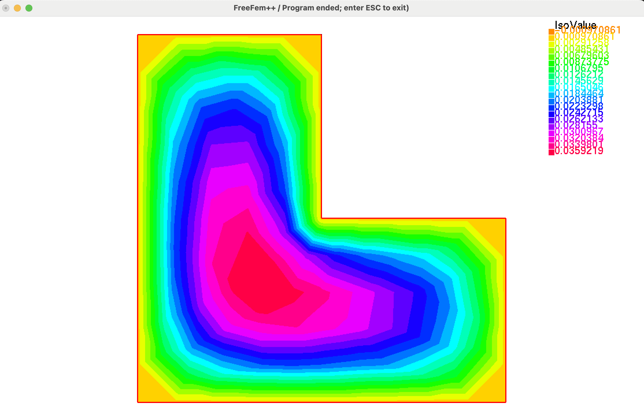
Fig. 1.11 Outcome of the \(\texttt{plot}\) command in \(\texttt{FreeFem}\).
1.5.2. A simple and efficient visualization tool: \(\texttt{medit}\)
The open-source software \(\texttt{medit}\) is a simple and efficient tool for displaying a mesh \(\calT_h\) and a \(\mathbb{P}_1\) function \(u\), supplied by its values at the vertices of \(\calT_h\). It can be used either directly within the \(\texttt{FreeFem}\) environment, or as a stand-alone program. We describe in this section a few important features of \(\texttt{medit}\), referring to the online documentation for a more advanced use.
Still in the context of the calculation of the solution \(u\) to the Laplace equation (1.22) on a mesh \(\calT_h\) considered in Section 1.4.2, \(\texttt{medit}\) can be used to visualize \(\calT_h\) and \(u\) through the following \(\texttt{FreeFem}\) syntax:
/* Load medit library */
load "medit"

[...]

/* Display mesh T_h and solution u */
medit("u", Th, u);
An alternative, more flexible means to use \(\texttt{medit}\) is to call it outside of \(\texttt{FreeFem}\), via command lines; most installations of \(\texttt{FreeFem}\) indeed come along with a fully-fledged installation of \(\texttt{medit}\). The latter can be called by using the following command line in the console:
ffmedit domain.mesh
Here, it is understood the the current directory contains a mesh file \(\texttt{domain.mesh}\) for the domain; if one additionally wishes to displaya solution attached to its vertices, the values of the latter must be contained in another file \(\texttt{domain.sol}\), i.e. sharing the same name as the mesh, with the different extension \(\texttt{.sol}\). In most situations, it is not necessary to understand the structures of \(\texttt{.mesh}\) and \(\texttt{.sol}\) files, since they can be read and saved by \(\texttt{FreeFem}\) functions; the curious or expert reader can find more information related to this structure in Section 1.6.3.
Let us illustrate visualization with \(\texttt{medit}\) with the mesh \(\calT_h\) and the solution \(u\) to the Laplace equation, tackled in Section 1.4.2. At first, in the \(\texttt{FreeFem}\) script, the mesh \(\calT_h\) and the \(\P_1\) finite element function \(u\) are saved as \(\texttt{.mesh}\) and \(\texttt{.sol}\) files, thanks to the following lines:
/* medit must be loaded to use savesol */
load "medit"

[...]

/* Display and save the result */
savemesh(Th,"Lshape.mesh");
savesol("Lshape.sol",Th,u);
We then call \(\texttt{medit}\) via the following console command:
ffmedit Lshape.mesh
A window opens, as depicted in Fig. 1.12.
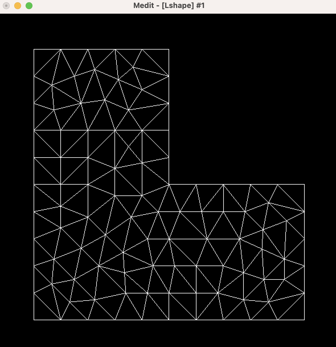
Fig. 1.12 Calling \(\texttt{medit}\) with the console.
Several keyboard shorthands then allow to act on the graphical rendering:
\(\texttt{b}\) switches the background color from black to white, and conversely;
\(\texttt{o}\) displays the isolines of the solution file;
\(\texttt{p}\) displays the color scale, see Fig. 1.13 (a);
\(\texttt{m}\) displays the values of the solution with a color filling rendering, as in Fig. 1.13 (b);
\(\texttt{k}\) reveals the 3d graph of the solution; using the left click allows to change the view, see Fig. 1.13 (c).
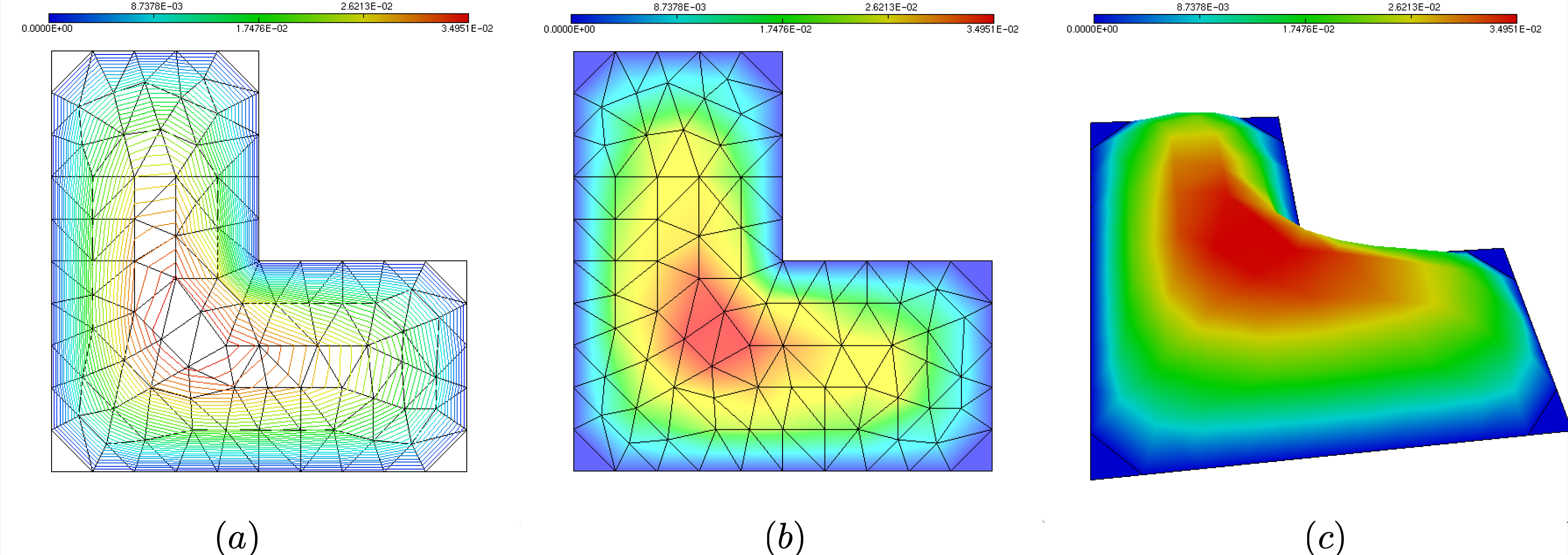
Fig. 1.13 A few basic commands in \(\texttt{medit}\): (a) Displaying the isolines of the solution and the color palette; (b) Using a color fill rendering; (c) Visualizing the graph of the solution.
\(\texttt{Medit}\) also enjoys convenient functionalities to access the values of the solution \(u\) at specific entities in the mesh:
Clicking on a triangle with \(\texttt{shift}\) reveals the number of the triangle, of its three vertices, and the values of the solution at those, see Fig. 1.14 (top).
Clicking on a vertex with \(\texttt{command} + \texttt{shift}\) shows the value of the solution at this vertex, see Fig. 1.14 (bottom).
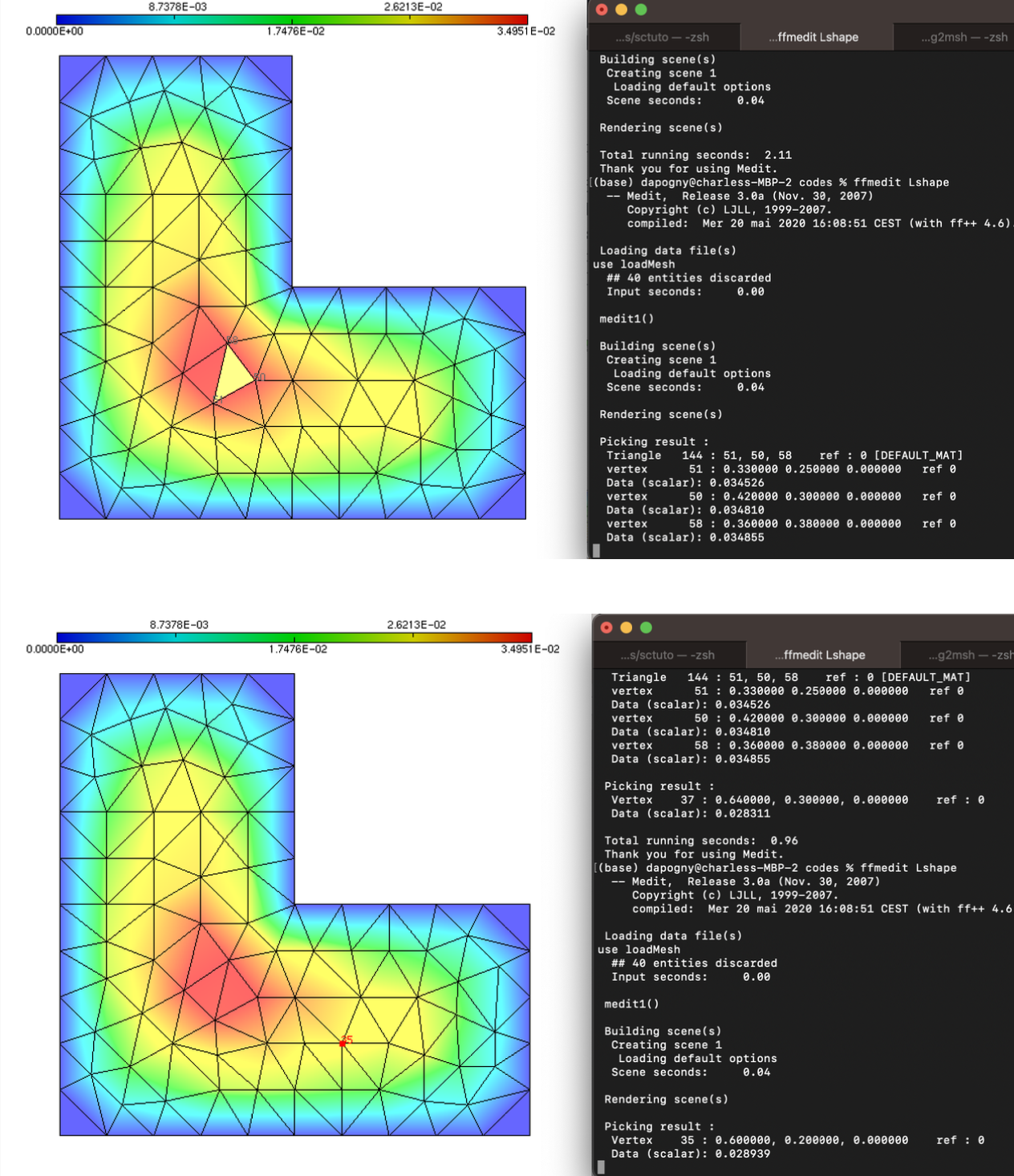
Fig. 1.14 (Top) Clicking on a triangle to display the numbers of its vertices and the values of the attached solutions; (bottom) Clicking on a vertex to display its number and the value of the attached solution.
A few additional features of \(\texttt{medit}\) rely on the use of a parameter file. The latter must be called \(\texttt{DEFAULT.medit}\); it is written by using any text editor, and it should be placed in the repository where \(\texttt{medit}\) is called – which may differ from the repository where the visualized files are located. Its syntax is very simple, and an example of such file can be downloaded here. This file is primarily used to customize the color scale for the displayed values of the solution: to achieve this, the keyword \(\texttt{palette}\) is used, and 5 reference values are supplied for the interpolation of the color scale, see Fig. 1.15.
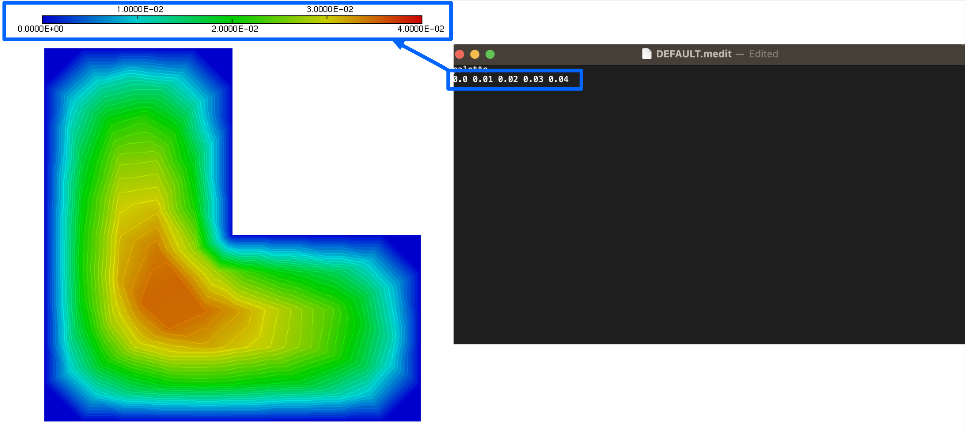
Fig. 1.15 The 5 supplied values under the keyword \(\texttt{palette}\) in the \(\texttt{DEFAULT.medit}\) file are those between which the color scale in the solution plot is interpolated.
Remark 1.9
Additional features of \(\texttt{medit}\) will be described in subsequent parts of this book:
Section 2.7.2 deals with the vizualization of meshes and solutions in 3d;
Section 3.2.2.2 is devoted to the vizualization of vector fields.
1.5.3. Creating animated \(\texttt{.gif}\) files using \(\texttt{medit}\)
The software \(\texttt{medit}\) makes it possible to create beautiful animated gifs with the outputs of numerical simulations. We illustrate this feature with the example of Section 1.4.4, dealing with the solution of the unsteady Laplace equation (1.25).
Let us recall that the solution of (1.25) was addressed by decomposing the total time interval \((0,T)\) into several subintervals \((t^n,t^{n+1})\), \(n=0,\ldots,N_1\); the values \(u^n(\x)=u(t^n,\x)\) of the solution \(u(t,\x)\) at the intermediate times \(t^n\) are computed and stored, via a sequence of \(\texttt{COMMON_NAME}.i.mesh\) files for the mesh of the computational domain \(\Omega\) and \(\texttt{COMMON_NAME}.i.sol\) files for the values of \(u^i\), \(i=1,\ldots,N\):
/* Load medit library */
load "medit"

[...]

/* Main loop */
for (int it=0; it<99; it++) {

  [...]

  /* Save solution */
  savemesh("heat."+(it+1)+".mesh");
  savesol("heat."+(it+1)+".sol",Th,u);
}
The execution of this code produces a sequence of \(100\) mesh files \(\texttt{heat.1.mesh}\), …, \(\texttt{heat.100.mesh}\) (which are, in the present case all identical) and \(100\) associated solutions \(\texttt{heat.1.sol}\), …, \(\texttt{heat.100.sol}\). These can be all read all visualized with \(\texttt{medit}\) as a sequence, via the following console command:
medit heat -a 1 100
After setting the rendering preferences (such as the background color, etc.), one may select the option \(\texttt{Toggle ImgSave}\) from the right-click menu, followed by \(\texttt{Play sequence}\); the sequence of meshes and solutions is played and each instance is saved as an image.
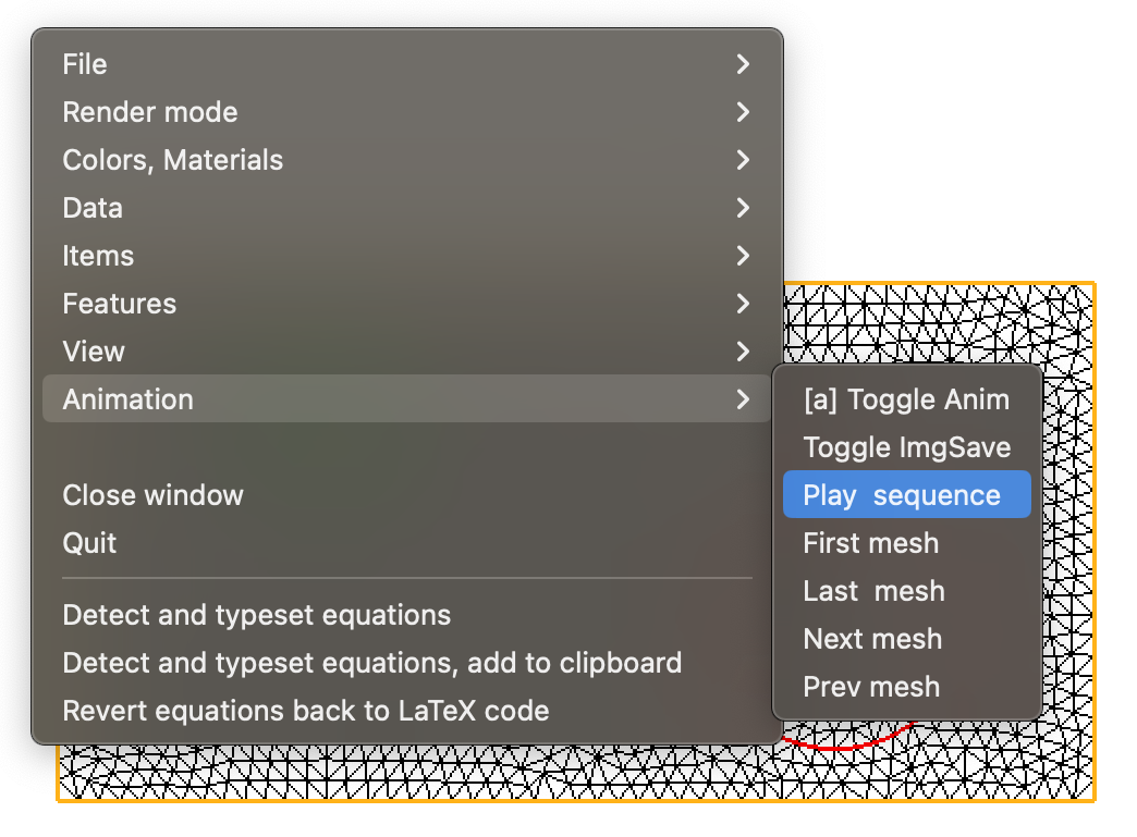
Fig. 1.16 Creating an animation with \(\texttt{medit}\) from a series of meshes and solutions.
The process output a series of \(\texttt{.ppm}\) image files: \(\texttt{heat.1.ppm}\), …, \(\texttt{heat.100.ppm}\). The latter can now be converted into a single \(\texttt{.gif}\) file. To this end, one may use, for instance the open-source software suite \(\texttt{ImageMagick}\); once the latter is installed, the following command achieves the desired purpose:
convert -loop 1 -delay 20 heat.?.ppm heat.??.ppm heat.???.ppm output.gif
Here, the option \(\texttt{-loop}\: 1\) indicates that the animation stops at the last image; if one wishes instead to repeat the animation indefinitely, this must be replaced with the option \(\texttt{-loop} \: 0\)). The option \(\texttt{delay}\) sets the delay between frames. The final result is depicted on Fig. 1.17.
Fig. 1.17 Animation of the solution to the unsteady Laplace example in Section 1.4.4.