1.9. The Laplace equation with pure Neumann boundary conditions

This section deals with the pure Neumann problem for the Laplace operator. A comprehensive reference about this issue is the journal article [BL05].

Let us consider the following boundary-value problem for the Laplace operator:

(1.33)\[\begin{split}\text{Search for } u \text{ s.t. } \left\{ \begin{array}{cl} -\Delta u = f & \text{in } \Omega, \\ \frac{\partial u}{\partial n} = 0 & \text{on } \partial \Omega. \end{array} \right.\end{split}\]

Here, the source \(f\) belongs to the space \(L^2(\Omega)\). The considered Neumann conditions are homogeneous, but inhomogeneous conditions could be analyzed by similar considerations.

1.9.1. A bit of theory

One subtle point about the pure Neumann problem (1.33) is that it is not necessarily well-posed. This is easily seen by multiplying both sides of the main equation by the constant function \(1\) and using the Green’s formula, which yields:

(1.34)\[\int_\Omega f(\x) \:\text{d} \x = 0.\]

This equality is a "compatibility condition", bearing only on the data \(f\) of the problem (1.33). If it is not satisfied, (1.33) cannot possibly have a solution.

On the other hand, when a solution \(u\) to (1.33) exists, it cannot be unique since then any function of the form \(u + c\), where \(c\) is a real constant, is obviously also a solution.

These evidences of the ill-posedness of (1.33) are actually two sides of the same coin. They actually reflect a very general phenomenon called Fredholm alternative: loosely speaking, the more numerous the compatibility conditions to be satisfied by the data for existence of a solution, the higher the dimension of the kernel of the problem.

Without entering any further into this deep mathematical topic, let us assume that the considered source \(f\) satisfies (1.34), and let us proceed formally to derive a variational formulation for (1.33), along the lines of Section 1.2. Because the solution \(u\) to (1.33) will be defined up to a constant, we search for one such solution \(u\) satisfying \(\int_\Omega u(\x) \:\d \x = 0\). Formally multiplying the main equation in (1.33) by a smooth test function \(v \in \calC^\infty(\overline\Omega)\), then applying the Green’s formula, we obtain:

\[\int_\Omega \nabla u \cdot \nabla v \:\d \x = \int_\Omega fv \:\d \x.\]

Besides, it is enough to assume that this relation holds true only for test functions \(v\) satisfying \(\int_\Omega v \:\d\x=0\), since it is obviously satisfied for \(v=1\), owing to (1.34). Since the differential operator at the left-hand side involves first-order partial derivatives of \(u\) and \(v\), we are led to consider the functional space

(1.35)\[V := \left\{ v \in H^1(\Omega) \text{ s.t. } \int_\Omega v \: \d \x = 0 \right\},\]

equipped with the norm \(\lvert\lvert \cdot \lvert\lvert_{H^1(\Omega)}\). These formal considerations lead us to introduce the following variational problem:

(1.36)\[\text{Search for } u \in V \text{ s.t. } \forall v \in V, \quad \int_\Omega \nabla u \cdot \nabla v \:\d \x = \int_\Omega f v \:\d \x.\]

The well-posedness of (1.36) is the subject of the next proposition, whose proof is left as an exercise.

Proposition 1.13

Let \(f \in L^2(\Omega)\) be a given source term. Then the variational problem (1.36) is well-posed.

Exercise

Prove proposition 1.13 thanks to the Lax-Milgram theorem.

(Hint: The coercivity of the bilinear form at the right-hand side of (1.36), rests on the Poincaré-Wirtinger inequality .)

Remark 1.12

The compatibility condition (1.34) is not needed to guarantee the well-posedness of (1.36). It however ensures that the variational solution \(u\) is also solution to the original boundary-value problem (1.33) in a suitable sense. Indeed, arguing as in remark 1.3 and without entering into details, one can show that \(u\) is the unique \(H^1(\Omega)\) function satisfying

\[\begin{split}\left\{ \begin{array}{cl} -\Delta u = f - \frac{1}{\lvert \Omega \lvert}\int_\Omega f(\x) \:\d \x & \text{in } \Omega, \\ \frac{\partial u}{\partial n} = 0 & \text{on } \partial \Omega. \end{array} \right.\end{split}\]

where the main equation is understood in the sense of distributions. Note that its right-hand side satisfies the compatibility condition (1.34) and that it coincides with the original source term \(f\) provided the latter satisfies (1.34).

1.9.2. Two different numerical resolution methods

Although rigorous, the mathematical framework developed in the previous Section 1.9.1 does not easily lend itself to numerical implementation. Indeed, the Finite Element discretization of the functional space (1.35), featuring functions with vanishing integral, is awkward. In the following, we describe two different mathematical and numerical approaches for the numerical resolution of (1.33).

1.9.2.1. The penalization method

Let \(\e\) be a "small" parameter. We propose to approximate the solution \(u\) to (1.33) by that \(u_{\e}\) to the following problem:

(1.37)\[\begin{split}\text{Search for } u_{\e}\:\: \text{ s.t. }\:\: \left\{\begin{array}{cl} -\Delta u +\e u= f & \text{in } \Omega, \\ \frac{\partial u_{\e}}{\partial n} = 0 & \text{on } \partial \Omega. \end{array} \right.\end{split}\]

Intuitively, the above boundary-value problem is a slightly modified version of (1.33) where a small \(0^{\text{th}}\) order term is added to the main equation. A variational formulation for this problem reads:

(1.38)\[\text{Search for } u_{\e} \in H^1(\Omega) \text{ s.t. } \forall v \in H^1(\Omega), \quad \int_\Omega \nabla u_{\e} \cdot \nabla v \:\d \x + \e \int_\Omega u_{\e} v \:\d \x = \int_\Omega f v \:\d \x.\]

A standard application of the Lax-Milgram theory shows that this variational problem is well-posed: indeed, the added \(0^{\text{th}}\) order term makes the bilinear form at the left-hand side coercive.

This penalization approach is made rigorous by the following proposition.

Proposition 1.14

Let \(f \in L^2(\Omega)\) satisfy the compatibility condition (1.34). The solution \(u_{\e} \in H^1(\Omega)\) to the penalized Laplace equation (1.37) converges to the solution \(u\) of the pure Neumann problem (1.33):

\[\lvert\lvert u_{\e} - u \lvert\lvert_{H^1(\Omega)} \xrightarrow{\e \to 0} 0.\]

Proof

The proof uses results about weak convergence.

At first, taking \(v=1\) in the variational formulation (1.38) for \(u_\e\), we see immediately that \(\int_\Omega u_{\e} \:\d\x =0\), because \(f\) satisfies (1.34).

Now, taking \(v=u_{\e}\), we obtain, in particular:

\[\int_{\Omega} \lvert \nabla u_{\e} \lvert^2 \:\d \x \leq C \lvert\lvert f \lvert\lvert_{L^2(\Omega)} \lvert\lvert u _\e\lvert\lvert_{L^2(\Omega)}.\]

The Poincaré-Wirtinger inequality then implies that \(u_{\e}\) is bounded in \(H^1(\Omega)\). Owing to proposition 6.2, we can thus extract a subsequence \(\e_n\) of the \(\e\) such that:

\[u_{\e_n} \to u_* \text{ weakly in } H^1(\Omega), \text{ for a certain limit function }u_*.\]

Passing to the weak limits in the variational problem (1.38) and in the relation \(\int_\Omega u _{\e_n} \:\d x\ =0\), we see that:

\[\forall v \in H^1(\Omega), \quad \int_\Omega \nabla u_{*} \cdot \nabla v \:\d\x = \int_\Omega fv \:\d\x, \text{ and } \int_\Omega u_* \:\d\x=0, \]

i.e. \(u_*\) is the unique solution to the pure Neumann problem in the space \(V\) defined by (1.35). Invoking a classical argument about the uniqueness of the limit, we conclude that the whole sequence \(u _\e\) converges to \(u\) weakly in \(H^1(\Omega)\).

To conclude, we have to prove that this convergence is actually strong. To achieve this, we just expand the square:

\[\begin{split}\begin{array}{ccl} \displaystyle\int_\Omega \lvert \nabla u_{\e} -\nabla u_* \lvert^2 \:\d\x &=& \displaystyle\int_\Omega \lvert \nabla u _\e \lvert^2 \:\d\x + \displaystyle\int_\Omega \lvert \nabla u \lvert^2 \:\d\x - 2 \displaystyle\int_\Omega \nabla u _\e \cdot \nabla u \:\d\x \\ &=& \displaystyle\int_\Omega f u _\e \:\d x + \displaystyle\int_\Omega f u \:\d \x - 2 \displaystyle\int_\Omega f u _\e \:\d \x, \end{array}\end{split}\]

where we have used both variational problems (1.38) and (1.36) with \(u\) and \(u _\e\) as test functions, respectively. Eventually, the right-hand side of the above equality tends to \(0\) as \(\e \to 0\) because of the weak \(H^1(\Omega)\) convergence of \(u_\e\) to \(u\), which ends the proof.

1.9.2.2. The constrained optimization method

In this section, we develop an alternative viewpoint about the variational problem (1.36), which is inspired by constrained optimization theory, a subject whose basic stakes are recalled in Section 6.5.

Let us recall that \(V\) stands for the space of functions in \(H^1(\Omega)\) with vanishing average on \(\Omega\), see (1.35). The energy version of the Lax-Milgram theorem in lemma 1.1 states that \(u\) is the unique solution to the following energy minimization problem:

\[\min_{v \in V} E(v), \text{ where } E(v) := \frac12 \int_\Omega \lvert \nabla v\lvert^2 \:\d \x - \int_\Omega fv \:\d \x.\]

Let us reformulate this as a constrained optimization problem:

\[\min_{v \in H^1(\Omega)} E(v) \text{ s.t. } \int_\Omega v \:\d x =0. \]

The necessary and sufficient optimality condition for this problem states that a solution \(u \in H^1(\Omega)\) to the latter should satisfy:

\[\exists \lambda \in \R, \text{ s.t. } \forall v \in H^1(\Omega), \quad \int_\Omega \nabla u \cdot \nabla v \:\d \x - \int_\Omega fv \:\d\x + \lambda \int_\Omega v \:\d \x = 0.\]

In particular, this relation should hold true for \(v=1\), which implies that the Lagrange multiplier \(\lambda\) necessarily equals:

\[\lambda = \frac{1}{\lvert\Omega\lvert} \int_\Omega f(\x) \:\d\x. \]

It follows that \(u\) is thus solution to the variational problem:

\[\text{Search for } u \in V, \text{ s.t. } \forall v \in V, \quad \int_\Omega \nabla u \cdot \nabla v \:\d \x = \int_\Omega \widetilde{f} v \:\d\x, \]

where \(\widetilde f := f - \frac{1}{\lvert\Omega\lvert}\int_\Omega f\:\d\x\) is the \(0\) averaged version of \(f\). In other words, \(u\) is the unique solution in \(V\) to the version of (1.33) featuring the \(0\) averaged right-hand side \(\widetilde{f}\). In particular, if \(f \in L^2(\Omega)\) satisfies the condition (1.34), the solution \(u\) to (1.33) can be calculated by searching for the unique pair \((u,\lambda) \in H^1(\Omega) \times \R\) satisfying the following variational problem:

\[\begin{split}\text{Search for } (u,\lambda) \in H^1(\Omega) \times \R \text{ s.t. } \forall (v,\mu) \in H^1(\Omega) \times \R, \quad \left\{ \begin{array}{l} \displaystyle\int_\Omega \nabla u \cdot \nabla v \:\d \x + \lambda \displaystyle\int_\Omega v \:\d \x = \displaystyle\int_\Omega fv \:\d\x, \\ \mu \displaystyle\int_\Omega u \:\d\x = 0, \end{array} \right.\end{split}\]

or equivalently:

(1.39)\[\text{Search for } (u,\lambda) \in H^1(\Omega) \times \R \text{ s.t. } \forall (v,\mu) \in H^1(\Omega) \times \R, \quad \int_\Omega \nabla u \cdot \nabla v \:\d \x + \lambda \int_\Omega v \:\d \x + \mu \int_\Omega u \:\d\x = \int_\Omega fv \:\d\x.\]

1.9.3. Implementation of the pure Neumann problem

We exemplify the resolution of the pure Neumann problem (1.33) with an example. The implementation of the penalization strategy of Section 1.9.2.1 is simple enough, and it is left as an exercise.

Exercise

Implement the penalization approach in Section 1.9.2.1 to solve the pure Neumann problem (1.33).

The solution based on the constrained optimization viewpoint of Section 1.9.2.2 is slightly more involved. The assembly of the Finite Element problem (1.39), posed over the product space \(H^1(\Omega) \times \R\), requires handling the Finite Element matrices associated to the three components of its left-hand side. This can be realized by using the syntax elements of Section 1.7.1, as described in the following listing. The complete numerical implementation of both approaches is proposed here, and the numerical results are presented on Fig. 1.24.

/* Resolution of the problem using Lagrange multipliers */
int nv = Vh.ndof;

/* Bilinear form for the Laplace equation */
varf varlap(u,v) = int2d(Th)(dx(u)*dx(v)+dy(u)*dy(v));

/* Bilinear form for the additional np*1 block */
varf vb(u,v) = int2d(Th)(1.0*v);

matrix A = varlap(Vh,Vh); // matrix with size nv*nv
real[int] B = vb(0,Vh); // Column bloc with size nv*1

/* Matrix of the augmented problem */
matrix Aa = [[A,B],[B',0]]; // B' = transpose of B

/* Construction of the right-hand side */
varf vrhs(u,v) =  int1d(Th,1)(gin*v) + int1d(Th,2)(gout*v);
real[int] b = vrhs(0,Vh);
real[int] ba(nv+1);
ba = [b,0.0];

/* Inversion of the augmented system */
set(Aa,solver=UMFPACK);
real[int] ua = Aa^-1*ba;
[u[],l] = ua;  // Comprehension of vector ua

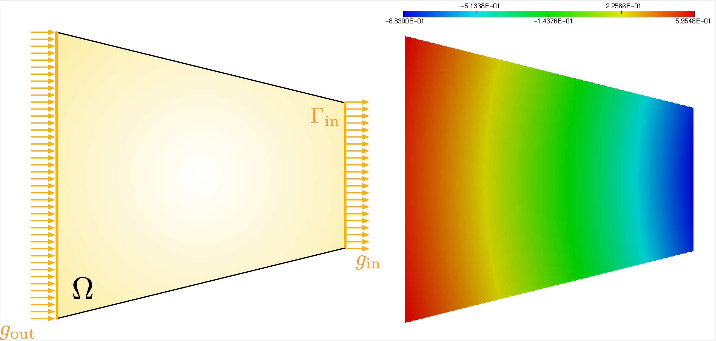
Fig. 1.24 Resolution of the pure Neumann problem (1.33); (Left) Setting of the test-case: heat is entering \(\Omega\) from the left boundary \(\Gamma_{\text{in}}\) with a flux \(g_{\text{in}}\) and is leaving \(\Omega\) from the right boundary \(\Gamma_{\text{out}}\) with a flux \(g_{\text{out}}\); (right) Plot of the solution.